2809
REconstruction of MR images acquired in highly inhOmogeneous fields using DEep Learning (REMODEL 2.0)1Department of Biomedical Engineering, Columbia University, New York, NY, United States, 2Columbia Magnetic Resonance Research Center, New York, NY, United States
Synopsis
The trade-off of a shorter MRI magnet design is having to compromise image quality due to reduced field homogeneity. Moreover, the sample induces unique field perturbations during the scan that can only be corrected if the exact field map is known. Here we proposed a DL model that synthesizes sample-specific field maps based on artifact-corrupted acquired images and the system’s field distribution. In the retrospective study, we obtained a mean NRMSE of 0.04 during testing between model output and the true field maps and found that using the model output for correction significantly reduced the artifacts on the images.
Introduction
MRI magnet design is a trade-off between accessibility parameters2 such as weight, dimensions, and cost and field homogeneity3,4. One approach to increase accessibility is to compromise the latter and consequently image quality to achieve compact, easier to site, and more affordable and reliable MRI systems3, 4. Field inhomogeneities pose challenges to the image acquisition principles, causing artifacts such as signal loss, geometrical distortions, and blurring5. Image reconstruction algorithms can correct these images utilizing a field map6-9. However, the field spatial distribution is unique during each acquisition as the sample introduces perturbations1. Most imaging protocols include the acquisition of the sample field map using a gradient echo sequence at two different echo times. Nevertheless, the correction quality of the images heavily depends on the quality of the field map itself10. In this work, we retrospectively test the ability of a deep learning model to synthesize the B0 field distortions caused by the sample based on the spatial distribution of an inhomogeneous system’s field and the corrupted acquired images.Methods
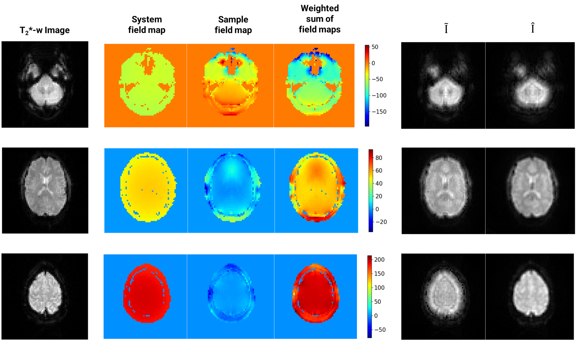
We simulated the effects of field inhomogeneity on a OpenNeuro dataset11 containing 100 resting-state images and field maps ($$$\omega_{sample}$$$). To obtain the field distribution of an inhomogeneous system ($$$\omega_{system}$$$), we acquired a field map using a uniform, cylindrical water phantom after turning off the Z and Z2 shims in a 3.0T Siemens Prisma Fit scanner. We used a weighted sum of the system and sample field maps to corrupt the functional images along a three-shot spiral trajectory with 11 ms readout duration following: $$\tilde{I}(r)=\mathcal{F}^{-1}\{S(t_k)e^{i(\omega_{system}(r)+\omega_{sample}(r))(TE+t_k)}\}$$ Where $$$r$$$ corresponds to the spatial coordinate vector, $$$S(t_k)$$$ the acquired signal kth time point, and $$$TE$$$ the echo time. The maximum inhomogeneity range achieved was ±400 Hz. After corruption, we corrected the resulting images using $$$\omega_{system}$$$ and obtained $$$\hat{I}$$$: $$\hat{I}(r)=\mathcal{F}^{-1}\{S(t_k)e^{-i\omega_{system}(r)(TE+t_k)}\}$$ Figure 1A summarizes the steps of data simulation. We leveraged the open-source tool OCTOPUS12 to corrupt and correct the images. The input to the model was a two-channel image: 1) the difference image $$$\tilde{I}-\hat{I}$$$ and, 2) its corresponding $$$\omega_{system}$$$ slice. The model’s output was $$$\omega_{sample}$$$ (Figure 1B). We preprocessed all images to be in the range [0,1], including the field data which was scaled to the absolute minimum and maximum frequency values of the dataset. The model architecture was the 7-block U-Net13 depicted in Figure 2. The data split divided the 14,405 simulated slices into 64-16-20% for training, validation, and testing. We chose Mean Squared Error (MSE) loss function and Root MSE (RMSE) as the performance metric. We tested the trained model performance on the test set and computed Normalized RMSE values between the predicted and true $$$\omega_{sample}$$$. Additionally, we corrected $$$\tilde{I}$$$ using the sum of the predicted $$$\omega_{sample}$$$ and $$$\omega_{system}$$$ and computed NRMSE between the result and the original functional slice.Results
Figure 3 displays representative simulation inputs, outputs, and corresponding field maps. The system field map is substantially homogeneous in-plane and the frequency value of each slice increases along the axial direction. This affects the weighted sum of field maps and consequently the severity of corruption in $$$\tilde{I}$$$, which worsens for the slices near the edges of the Field Of View (FOV) compared to the center slice. After 100 epochs, the MSE and RMSE were reduced to 3.58%/18.92% for training and 11.14%/33.38% for validation. These values are relative to the initial errors of the untrained model. The difference between predicted and true outputs for the test set showed a mean NRMSE=0.04±0.18. The difference between $$$\tilde{I}$$$ corrected using the predicted and the original functional images yielded a mean NRMSE=2.36±1.82.Discussion
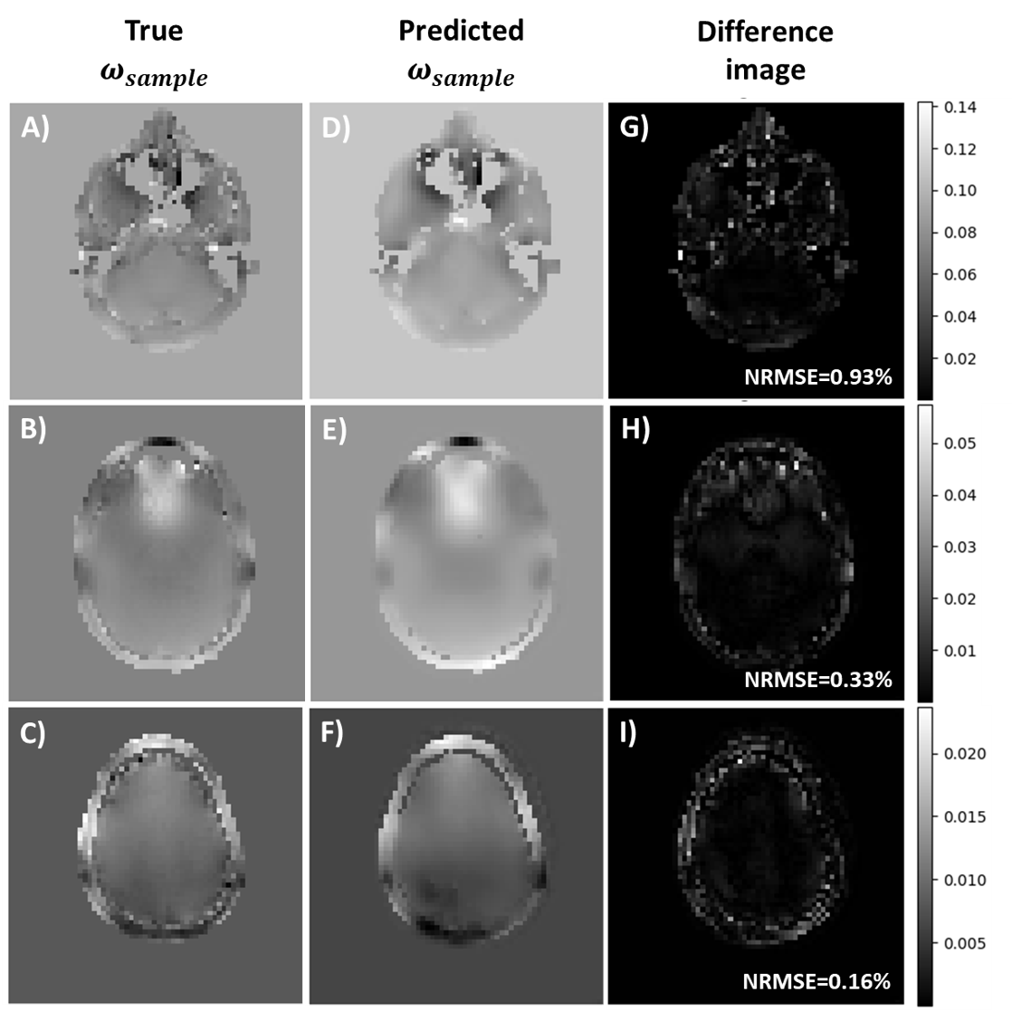
We hypothesize that by feeding the model the difference between $$$\tilde{I}$$$ and $$$\hat{I}$$$ and the system field map, it is learning the relation between the field frequency values and the magnitude of the error in $$$\tilde{I}-\hat{I}$$$, corresponding to the sample-induced perturbations.Figure 4 compares true $$$\omega_{sample}$$$ against predicted $$$\omega_{sample}$$$ and shows the difference image between the two. Lower NRMSE values suggest that the model predicts better when the field map is smoother such as for top slices of the brain. In contrast, bottom slices containing air-tissue interfaces such as the frontal sinus region present rapid frequency fluctuations in the field map that are smoothened by the model, resulting in higher NRMSE values.
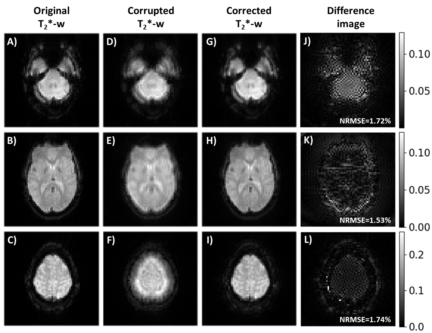
Figure 5 compares the original functional images and the image obtained after correcting $$$\tilde{I}$$$ with the sum of the system’s and predicted sample field map. As seen in Figure 3, $$$\tilde{I}$$$ is more severely artifacted for slices near the FOV edges where the system field map presents higher absolute frequency values. Thus, correction performance shows also higher NRMSE values in these cases compared to slices acquired near the magnet isocenter.
Conclusion
We have retrospectively trained, validated, and tested a DL model to synthesize sample-specific field maps from corrupted functional images acquired in the presence of a field inhomogeneity within ±400 Hz. Current and future experiments include explaining the working of the DL model, expanding the range of off-resonance frequencies, and prospective demonstrating the use on a 3D spiral fMRI acquisition at 3.0T.Acknowledgements
This study was funded [in part] by the Seed Grant Program for MR Studies and the Technical Development Grant Program for MR Studies of the Zuckerman Mind Brain Behavior Institute at Columbia University and Columbia MR Research Center site.References
- K. M. Koch, D. L. Rothman, and R. A. de Graaf, “Optimization of static magnetic field homogeneity in the human and animal brain in vivo,” Prog. Nucl. Magn. Reson. Spectrosc., vol. 54, no. 2, pp. 69–96, 2009.
- S. Geethanath and J. T. Vaughan, “Accessible magnetic resonance imaging: A review,” J. Magn. Reson. Imaging, vol. 49, no. 7, pp. 65–77, 2019.
- T. C. Cosmus and M. Parizh, “Advances in whole-body MRI magnets,” IEEE Trans. Appl. Supercond., vol. 21, no. 3, pp. 2104–2109, 2011.
- Y. Lvovsky, E. W. Stautner, and T. Zhang, “Novel technologies and configurations of superconducting magnets for MRI,” Supercond. Sci. Technol., vol. 26, no. 093001, 2013.
- M. Mullen and M. Garwood, “Contemporary approaches to high-field magnetic resonance imaging with large field inhomogeneity,” Prog. Nucl. Magn. Reson. Spectrosc., vol. 120–121, pp. 95–108, 2020.
- D. C. Noll, C. H. Meyer, J. M. Pauly, D. G. Nishimura, and A. Macovski, “A Homogeneity Correction Method for Magnetic Resonance Imaging with Time-Varying Gradients,” IEEE Trans. Med. Imaging, 1991.
- B. P. Sutton, D. C. Noll, and J. A. Fessler, “Fast, iterative image reconstruction for MRI in the presence of field inhomogeneities,” IEEE Trans. Med. Imaging, 2003.
- L. C. Man, J. M. Pauly, and A. Macovski, “Multifrequency interpolation for fast off-resonance correction,” Magn. Reson. Med., vol. 37, no. 5, pp. 785–792, 1997.
- V. J. Schmithorst, B. J. Dardzinski, and S. K. Holland, “Simultaneous correction of ghost and geometric distortion artifacts in EPI using a multi-echo reference scan,” IEEE Trans. Med. Imaging, vol. 20, no. 6, pp. 535–539, 2001.
- Z. Hu et al., “Distortion correction of single-shot EPI enabled by deep-learning,” Neuroimage, vol. 221, no. 117170, 2020.
- E. M. Gordon et al., “The Midnight Scan Club (MSC) dataset”. OpenNeuro, 2020. [Dataset] doi: 10.18112/openneuro.ds000224.v1.0.3
- M. Manso Jimeno, J. Vaughan, and S. Geethanath, “Off-resonance CorrecTion OPen soUrce Software (OCTOPUS),” J. Open Source Softw., vol. 6, no. 59, p. 2578, 2021.
- O. Ronneberger, P. Fischer, and T. Brox, “U-net: Convolutional networks for biomedical image segmentation,” in Lecture Notes in Computer Science (including subseries Lecture Notes in Artificial Intelligence and Lecture Notes in Bioinformatics), 2015.
Figures
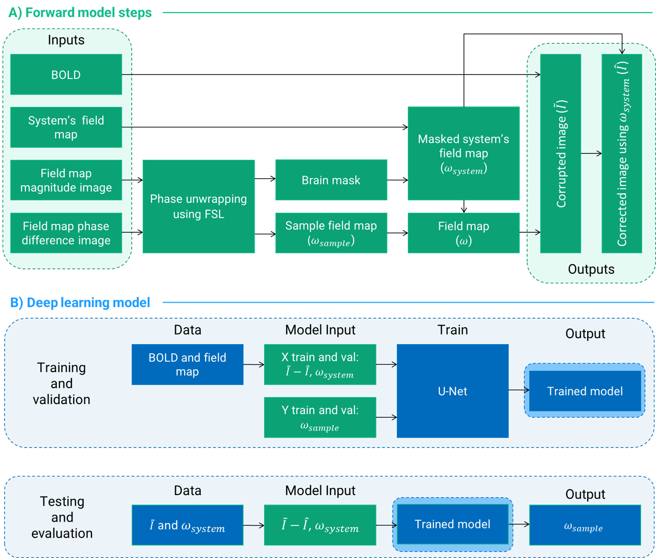
Figure 1: (A) Diagram of the field inhomogeneity artifacts simulation steps. B) Summary of the deep learning model inputs and output.

Figure 2: Diagram of the U-Net model architecture. Each block consisted of two convolutional layers with ReLU activation and a dropout layer in between. To achieve a single-channel output we added a single-filter with 1x1 kernel size convolutional layer at the end of the U-Net.