Introduction

MRI-Linac systems have been developed for radiotherapy treatments to enable adaptive tracking and localization of tumors [1]. The Australian 1T open bore MRI-Linac uses a split magnet with a 50 cm gap to facilitate treatment beam delivery and patient positioning [2]. However, the split bore configuration inevitably compromises B0 field homogeneity, which can cause image distortions and potentially misplaced radiation doses [3]. Spherical harmonic (SH) models can be used to characterize and correct geometric distortions [4]. However, the split magnet design exhibits more complex B0 inhomogeneity field, which requires higher SH terms compared with conventional MRI scanners. In this work, we develop a high-order SH model to correct B0 inhomogeneity induced distortions. A reverse gradient technique with a grid phantom was used to measure image deformation and SH coefficients describing the B0 field were iteratively calculated from measured phantom marker positions. Evaluated using phantom data acquired from Australian MRI-Linac scanner, a 10th order SH model reduces geometric displacement to less than 2 mm.

Methods

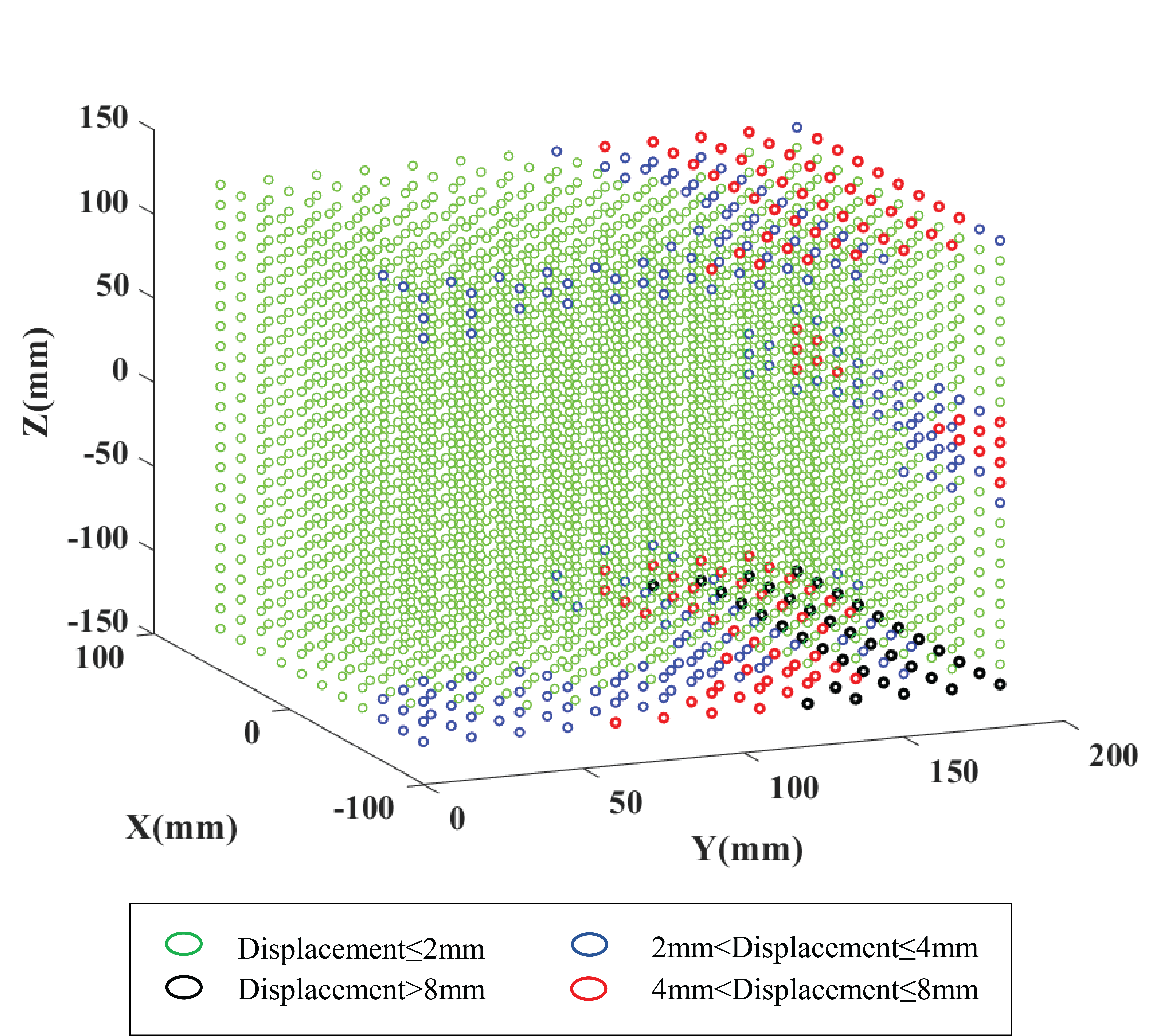
Due to gradient nonlinearity (GNL) and B0 inhomogeneity, the undistorted position L of an object can be found at location L⁺ with a positive encoding gradient and at location L^- with a negative encoding gradient, governed by the equations [5] below: $$\begin{equation}\begin{aligned}&L^{+}=L+\frac{d B_{L}(x, y, z)}{G_{L}}+\frac{d B_{0}(x, y, z)}{G_{L}}\;\;\;\;\;\;\;\;\;\;\;\;\;\;\;\;\;\;(1)\\&L^{-}=L+\frac{d B_{L}(x, y, z)}{G_{L}}-\frac{d B_{0}(x, y, z)}{G_{L}} \;\;\;\;\;\;\;\;\;\;\;\;\;\;\;\;\;\;(2)\end{aligned}\end{equation}$$ where dB_L and dB₀ represent gradient and B0 field perturbations, respectively. G_L denotes the gradient strength along L axis. The sign of spatial distortion $$$\frac{d B_{0}(x, y, z)}{G_{L}}$$$ caused by B0 field inhomogeneity is affected by gradient polarity differences and thus B0 inhomogeneity distortions can be extracted by averaging the displacements:$$\frac{L^{+}-L^{-}}{2}=\frac{d B_{0}(x, y, z)}{G_{L}}\;\;\;\;\;\;\;\;\;\;\;\;\;\;\;\;\;\;(3) $$ The inhomogeneous B0 field over the whole field of view (FOV) can be described by an SH model [6]:$$d B_{0}(L)=\sum_{n=0}^{N} \sum_{m=0}^{n} r^{n}(L) P_{n m}(\cos (\theta(L)))\left[A_{n m}^{k} \cos (m \emptyset(L))+B_{n m}^{k} \sin (m \emptyset(L))\right]\;\;\;\;\;\;\;\;\;\;\;\;\;\;\;\;\;\;(4)$$ where N and m represent the order and degree of SH models, respectively. $$$P_{n m}(\cdot)$$$ denotes the associated Legendre function. $$$A_{n m}^{k}$$$ and $$$B_{n m}^{k}$$$ are unknown SH coefficients of order N and degree m, which can be inversely calculated by the equation below:$$\underset{\left(A_{n m}^{k}, B_{n m}^{k}\right)}{\operatorname{argmin}}\left\|C\left\{L_{d i s}, (A_{n m}^{k},B_{n m}^{k})\right\}-L\right\|_{F}^{2} \;\;\;\;\;\;\;\;\;\;\;\;\;\;\;\;\;\;(5)$$ Where L_dis represents the distorted position caused only by B0 inhomogeneity which can be calculated by Eq. (3) and C{·} denotes the distortion-corrected position using our previously developed GNL-encoding method [7] based on the SH model. The Gauss-Newton (GN) [5] iteration was used to solve the minimization problem.
A 3D grid phantom was scanned on the Australian 1T MRI-Linac system with normal and reversed gradient encoding polarities to measure B0 inhomogeneity distortion, as shown in Figure 1. To cover the imaging area over a large diameter of spherical volume (DSV), the phantom center was shifted by 10cm from scanner isocenter along y direction. A total of 3289 markers were extracted from this measurement dataset in a FOV of 20 cm × 20 cm × 30 cm. These measured marker positions were used to inversely calculate SH coefficients with various orders based on Eq. (5). The sequence was turbo spin echo (TSE), image size = 130 × 110 × 192, resolution = 1.8 mm × 2 mm × 1.8 mm, TE/TR = 15 ms/5.1 s, and pixel bandwidth = 202 Hz. To test the proposed method, another testing phantom dataset was acquired with same imaging parameters, where the phantom was shifted by 2cm along y direction from the previous scan.

Results

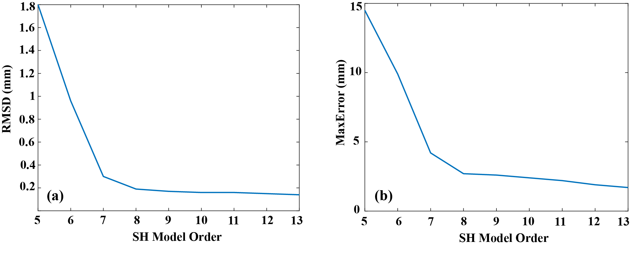
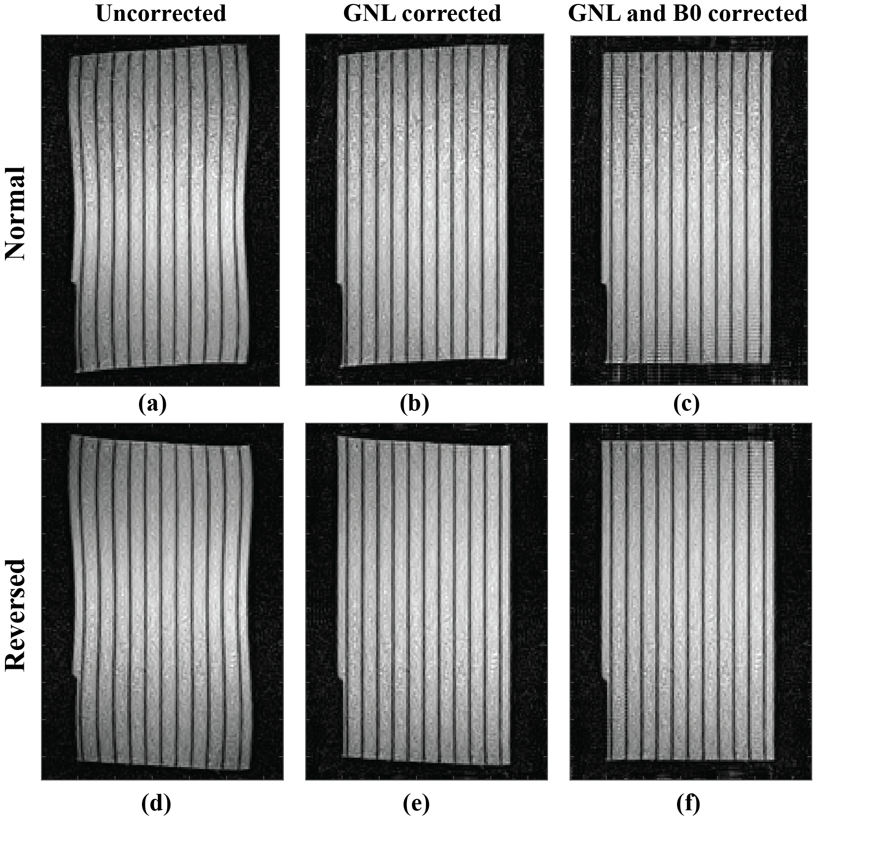
As shown in Figure 2, markers close to isocenter have distortion within 2mm, however at the edge area, displacement over 8mm is presented, indicating that B0 inhomogeneity is exacerbated with the distance from the isocenter. Figure 3 shows the root mean square deviation (RMSD) values and maximal error using SH models with different model orders. The RMSD value and maximum error change dramatically for orders from 5th to 8th and the difference is subtle for orders over 10th. Phantom images from the testing dataset acquired with both normal (a-c) and reversed gradient (d-f) polarities are shown in Figure 4. After GNL distortion correction using our previously developed EM model [7], residual distortions in Figure 4b and Figure 4e are only caused by B0 inhomogeneity. Geometric differences between Figure 4b and Figure 4e demonstrate that B0 inhomogeneity induced distortions are affected by gradient polarities. After applying the proposed method, distortions are almost invisible in Figure 4c and Figure 4f. Quantitatively, the maximal displacement is reduced from 12.2mm to 1.7mm on phantom images from the testing dataset before and after correction.

Discussion

The SH order determines the accuracy of the proposed method, and a 10th order model was utilized based on the RMSD and maximal error analysis in this study. B0 inhomogeneity distortion is dependent on sequence parameters [8] but can be predicted since the magnitude of distortion scales inversely with readout gradient strength, as shown in Eq. (1-2).

Conclusion

In this work, an SH model of up to 10th order is developed for B0 distortion correction on a 1T open bore MRI-Linac. Phantom results show that the geometric inaccuracy is within 2mm after correction, which will be used to improve the accuracy of MRI-Linac treatments.

References

[1] Pollard JM, Wen Z, Sadagopan R, Wang J, Ibbott GS. The future of image-guided radiotherapy will be MR guided. The British journal of radiology. 2017;90(1073):20160667.
[2] Keall PJ, Barton M, Crozier S. The Australian magnetic resonance imaging–linac program. Paper presented at: Seminars in radiation oncology2014.
[3] Baldwin LN, Wachowicz K, Fallone BG. A two‐step scheme for distortion rectification of magnetic resonance images. Medical physics. 2009;36(9Part1):3917-3926.
[4] Acquaviva, R., Mangione, S. and Garbo, G., 2018. Image-based MRI gradient estimation. Magnetic resonance imaging, 49, pp.138-144.
[5] Baldwin, L.N., Wachowicz, K., Thomas, S.D., Rivest, R. and Fallone, B.G., 2007. Characterization, prediction, and correction of geometric distortion in MR images. Medical physics, 34(2), pp.388-399.
[6] Tao S, Trzasko JD, Gunter JL, et al. Gradient nonlinearity calibration and correction for a compact, asymmetric magnetic resonance imaging gradient system. Phys Med Biol. 2017;62(2):N18-N31.
[7] Shan, S., Liney, G. P., Tang, F., Li, M., Wang, Y., Ma, H., ... & Crozier, S. (2020). Geometric distortion characterization and correction for the 1.0 T Australian MRI‐linac system using an inverse electromagnetic method. Medical physics, 47(3), 1126-1138.
[8] Walker, A., Liney, G., Holloway, L., Dowling, J., Rivest‐Henault, D. and Metcalfe, P., 2015. Continuous table acquisition MRI for radiotherapy treatment planning: distortion assessment with a new extended 3D volumetric phantom. Medical physics, 42(4), pp.1982-1991.