Introduction

Variable flip angle (VFA) T1-mapping and dynamic contrast enhanced (DCE) MRI are important for a range of oncological applications, including cancer detection, diagnosis, staging, and treatment evaluation [1-3].

Fat suppression (FS) in VFA T1-mapping and DCE-MRI would be beneficial, as the bright signal from fat can obscure the region of interest and prevent problems due to water-fat shift. In particular, radial acquisitions suffer from substantial streaking artefacts without FS.

However, FS-pulses disrupt the steady-state magnetization that is the basis for VFA T1-relaxometry and DCE modelling, and hence FS is barely applied in DCE [4, 5]. In fact, the QIBA guidelines advice against FS as converted contrast concentrations would be incorrect due to a wrong model for baseline T1 estimates as well as for converting the signal to concentration, both required for DCE [6]. If we can account for these FS pre-pulses in the T1-relaxometry and DCE modelling, we would enable FS and allow for pharmacokinetic modelling analysis in the presence of fat.

Therefore, we included the effect of a FS-pulse into the spoiled gradient echo (GRE) signal equation, used for relaxometry and DCE modelling.

Methods

Theory
Without FS pre-pulse, the signal equation for GRE sequences is [7]:

$$$S = M_0\sin{(FA)}\frac{1-\mathrm{e}^{{\frac{-TR}{T1}}}}{1-\mathrm{e}^{{\frac{-TR}{T1}}}\cos{(FA)}}$$$[Eq.1]

with $$$FA$$$ flip angle, $$$S$$$ signal, $$$M_0$$$ magnetization in z-direction, and $$$TR$$$ repetition time. When GRE is interleaved with spectral FS pre-pulses, the steady-state of water is interrupted with a longer TR during which additional T1-relaxation takes place. We assume that magnetization right before the FS-pulse ($$$M_{startFS}$$$) is equal to the magnetization after ($$$M_{endFS}$$$), except for T1-relaxation during the pulse:

$$$M_{endFS}=M_{startFS}+(M_0-M_{startFS})(1-E_{1,FS})$$$[Eq.2]

with $$$E_{1,FS}=\mathrm{e}^{-\frac{TR_{FS}}{T1}}$$$ where $$$TR_{FS}$$$ is the duration of the FS-pulse. Furthermore, the magnetization after a train of GRE pulses after the end of the FS-pulse is:

$$$M_k=M_{endFS}(E_1\cos⁡(FA))^{k-1}+M_0(1-E_1)\frac{(1-E_1)cos⁡(FA)^{k-1}}{1-E_1\cos⁡(FA)}$$$[Eq.3]

with $$$E_{1}=\mathrm{e}^{-\frac{TR}{T1}}$$$ and $$$n$$$ the number of excitations after FS. In particular, with $$$k$$$ excitations between FS-pulses, we find $$$M_{startFS}=M(k)$$$. By combining this with Eq. 2 and 3, the signal equation that takes into account FS is derived initially at $$$M_{endFS}$$$ . Then, with Eq. 3 again, the signal at $$$n$$$ excitations after FS is found:

$$$S=M_0\sin(FA)\left[\left[\left[\frac{(1-E_{1,FS})(E_1\cos⁡(FA))^{k-1}+(1-E_1)\frac{1-(E_1\cos⁡(FA))^{k-1}}{1-E_1\cos⁡(FA)}}{(1-E_{1,FS}(E_1\cos⁡(FA))^{k-1})}\right]E_{1,FS}+(1-E_{1,FS})\right](E_1\cos⁡(FA))^{n-1}+(1-E_1)\frac{1-(E_1\cos⁡(FA))^{n-1}}{1-E_1\cos⁡(FA)}\right]$$$[Eq.4]

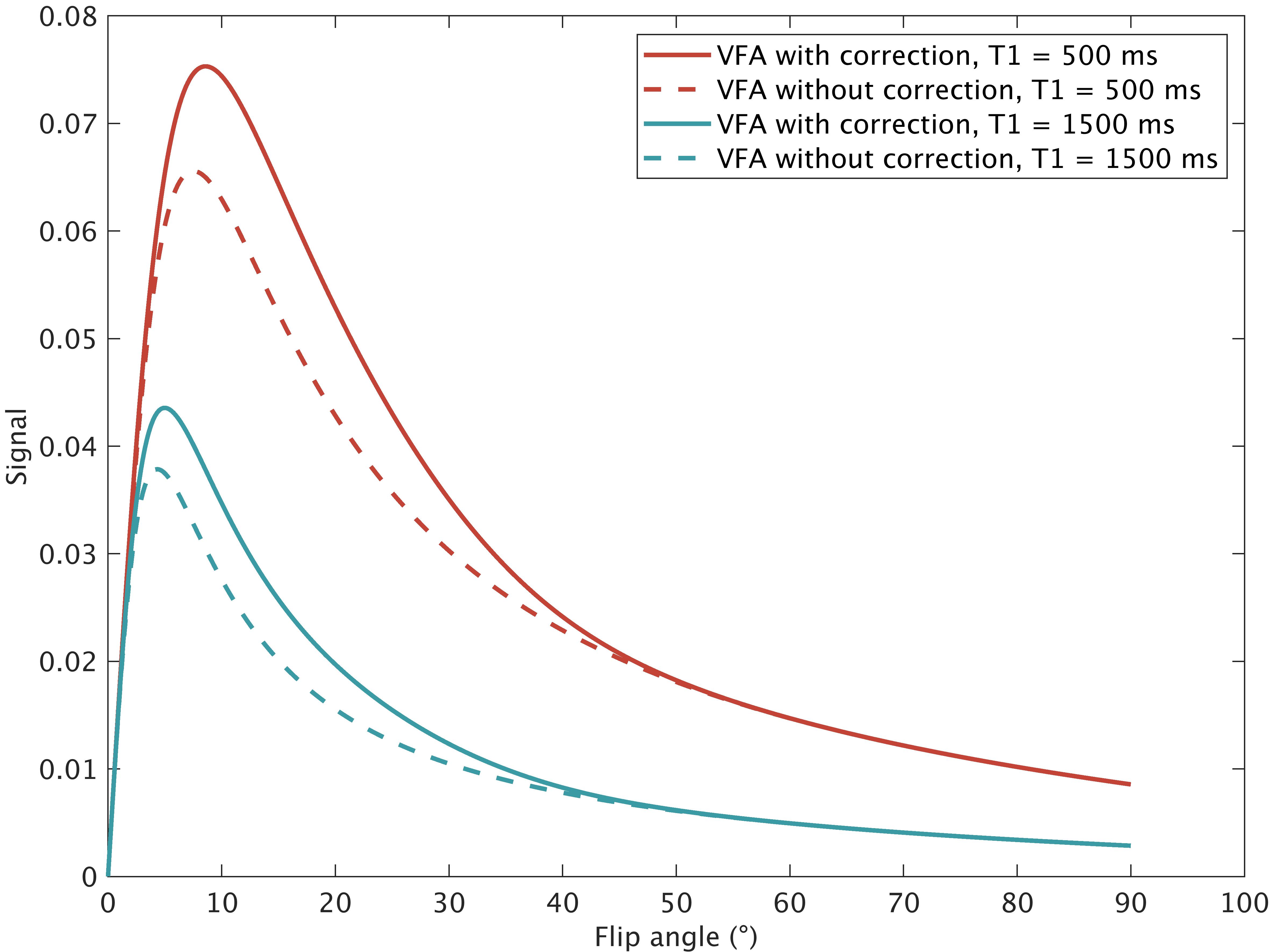
with $$$k$$$ the number of excitations between the FS-pulses. Assuming signal contrast is predominantly defined when the center of k-space is acquired, we can take $$$n=$$$ excitations until center of k-space to obtain the signal equation (Figure 1). Determining $$$n$$$ depends on acquisition parameters, including the k-space filling order, the partial-Fourier factor, start-up echoes and the shot-length.

Although these equations hold T1-mapping and for converting to contrast concentration in DCE, they are easiest validated using T1-mapping. Hence we focus on T1-relaxometry for this abstract.

Data
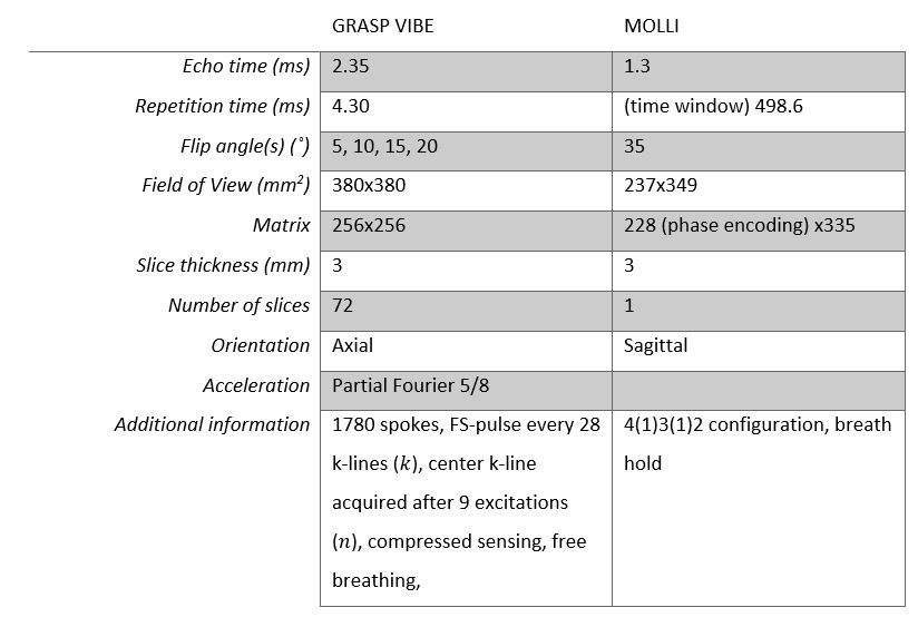
Five healthy volunteers, three ICU patients, and the NISTI system phantom (CaliberMRI, T1 reference values 10–1879ms) were imaged on a 1.5T MAGNETOM Sola (Siemens Healthineers) using a 32-channel body coil. T1-maps were obtained with a fat-saturated VFA GRASP method and conventional Modified Look-Locker (MOLLI), Table 1. For the phantom, a B1 map was acquired using the dual FA method [8] to correct the FAs for B1 inhomogeneities. T1 fitting for the MOLLI method was performed, after non-rigid motion correction, using qMRLAB in MATLAB 2021a [9]. For the VFA-GRASP method, an in-house fitting pipeline was developed in MATLAB 2021a based on Eq. 1 and 4. Fitted values were compared between results from the MOLLI and VFA GRASP methods versus the manufacturer-provided reference T1 values from the phantom using linear regression ($$$\alpha = 0.05$$$). In human subjects, results from different tissues were compared using Bland-Altman analysis (liver, spleen, and skeletal muscle).

Results

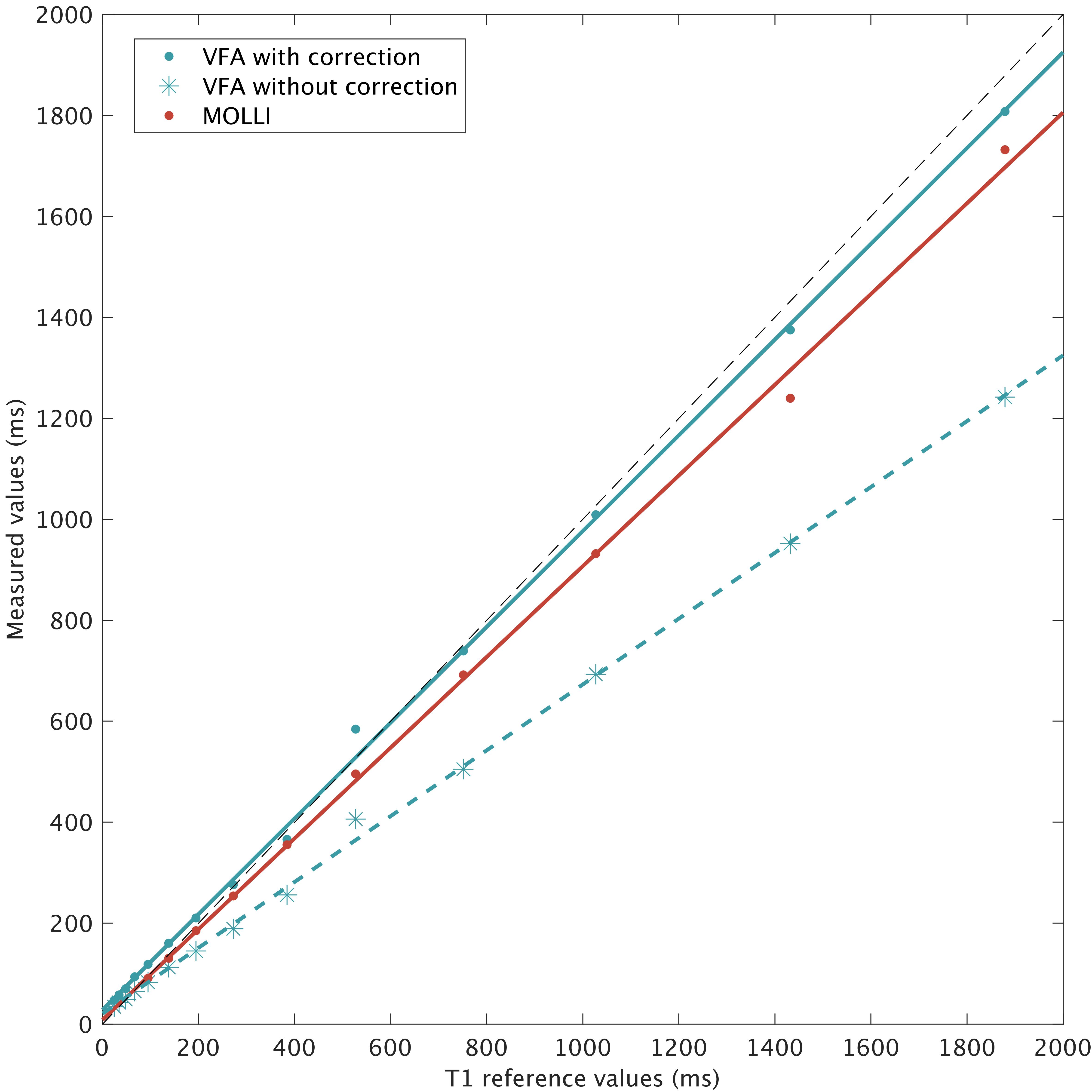
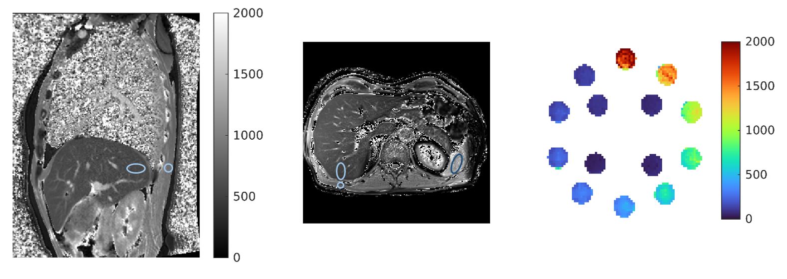
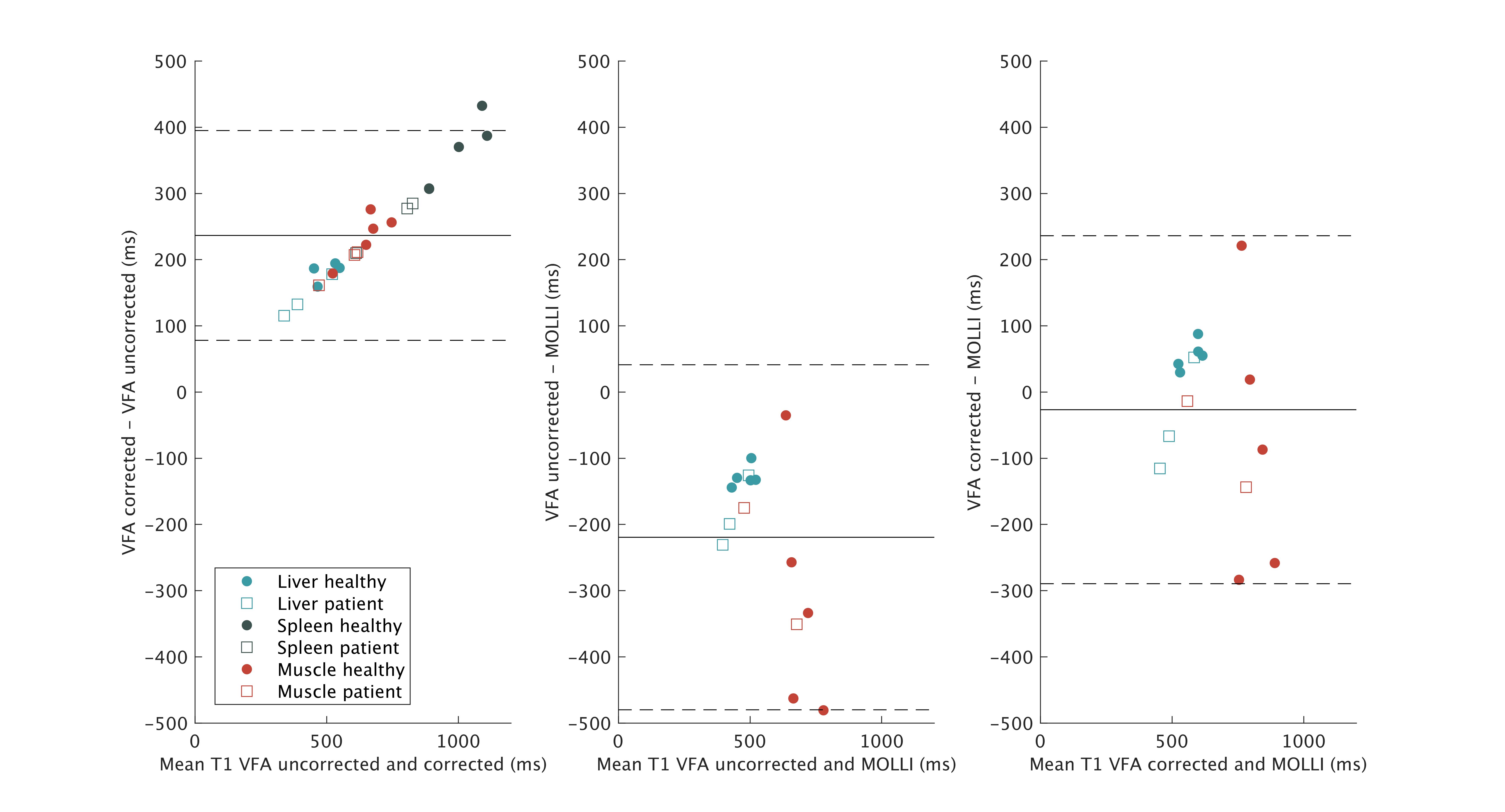
There was a good agreement for the corrected VFA method and MOLLI (slope 0.95 and 0.90 respectively) with the reference values (Figure 2), but notably worse agreement when not correcting for FS in VFA (slope 0.64). We successfully obtained T1-maps and regions of interest in the phantom and human subjects (Figure 3). There was a difference between the T1-values measured using the corrected VFA and MOLLI method (Figure 4), with a systematic difference of -25 ms (VFA - MOLLI), but this difference was larger (-219 ms) without correction for FS. Secondly, Figure 4 displays a linear bias between the uncorrected and corrected VFA methods.

Discussion

We introduced a novel VFA method that adopted GRASP and FS for T1-fitting and measured 3D T1-maps during free-breathing in healthy subjects and ICU patients. This method was more accurate than MOLLI in a phantom, and greatly outperformed the conventional VFA fit (Figure 2). In human subjects, the correction for FS improved the agreement with MOLLI. The overall agreement of the T1 values measured with MOLLI and the corrected VFA method were mediocre (limits of agreement -289ms, 236ms). We believe this reflects the shortcomings of our reference method MOLLI as, it is a 2D method with one slice only acquisition, imperfect breath-holding, and was acquired in a different orientation as the VFA.

Conclusion

We have presented a fat-suppressed VFA T1-mapping technique that yields accurate T1-values for relaxometry and DCE-MRI applications. This technique will enable T1-relaxometry and DCE in fatty regions and allow for quantitative imaging with GRASP.

Acknowledgements

None.