2692

Visualising and interacting with diffusion MRI microstructural models using FSL-DIVE

Michiel Cottaar¹, Nicole Eichert¹, Hossein Rafipoor¹, Amy Howard¹, Daniel Kor¹, Jiewon Kang¹, Pavan Chaggar^1,2, Ying-Qiu Zheng¹, Sean Fitzgibbon¹, and Saad Jbabdi¹
¹University of Oxford, OXFORD, United Kingdom, ²Mathematics, University of Oxford, Oxford, United Kingdom

Synopsis

We introduce FSL-DIVE, an interactive visualisation software for diffusion microstructure modelling. This software allows the user to (i) flexibly set up a multi-compartment microstructure model, including fibre orientation modelling and restricted diffusion, (ii) choose different acquisition parameters, (iii) change the model parameters and analyse the model behaviour through multiple bespoke plots, (iv) save the predicted data (including noise) for any specified acquisition scheme. We hope this tool may be useful for teaching diffusion microstructure modelling, for developing new models, or for getting a better understanding of existing models.

Introduction

Microstructure modelling is an exciting area of diffusion MR imaging. Biophysically inspired models are used to infer tissue microstructure correlates of diffusion MR signals, with the aim to provide specific and quantitative markers of tissue state. Many such models have been proposed to estimate brain tissue features such as soma size, axon diameter or fibre orientation and dispersion [1]. These microstructural models are typically composed of different compartments, each with specific geometric and diffusion properties, leading to a signature diffusion profile [2]. While fitting these complex models to diffusion data can hopefully yield more specific, interpretable quantities (e.g., axon diameter or density) than phenomenological models (e.g., tensor FA), it is also important to realise the limitations that these models can have. For example, they are a simplified version of reality, and they can be over-parameterised, which is problematic for parameter fitting [3]. In addition, it is important to understand the different experimental conditions under which these models can be useful. To help get a handle on diffusion microstructure models, we developed an open-source visualisation tool that allows the user to flexibly specify a multi-compartment diffusion model, change the model parameters, immediately observe their effect on the predicted signals, and flexibly alter the diffusion acquisition protocol. We hope that this tool will be useful for probing diffusion models, for developing new models, and for teaching.

Overview of the software

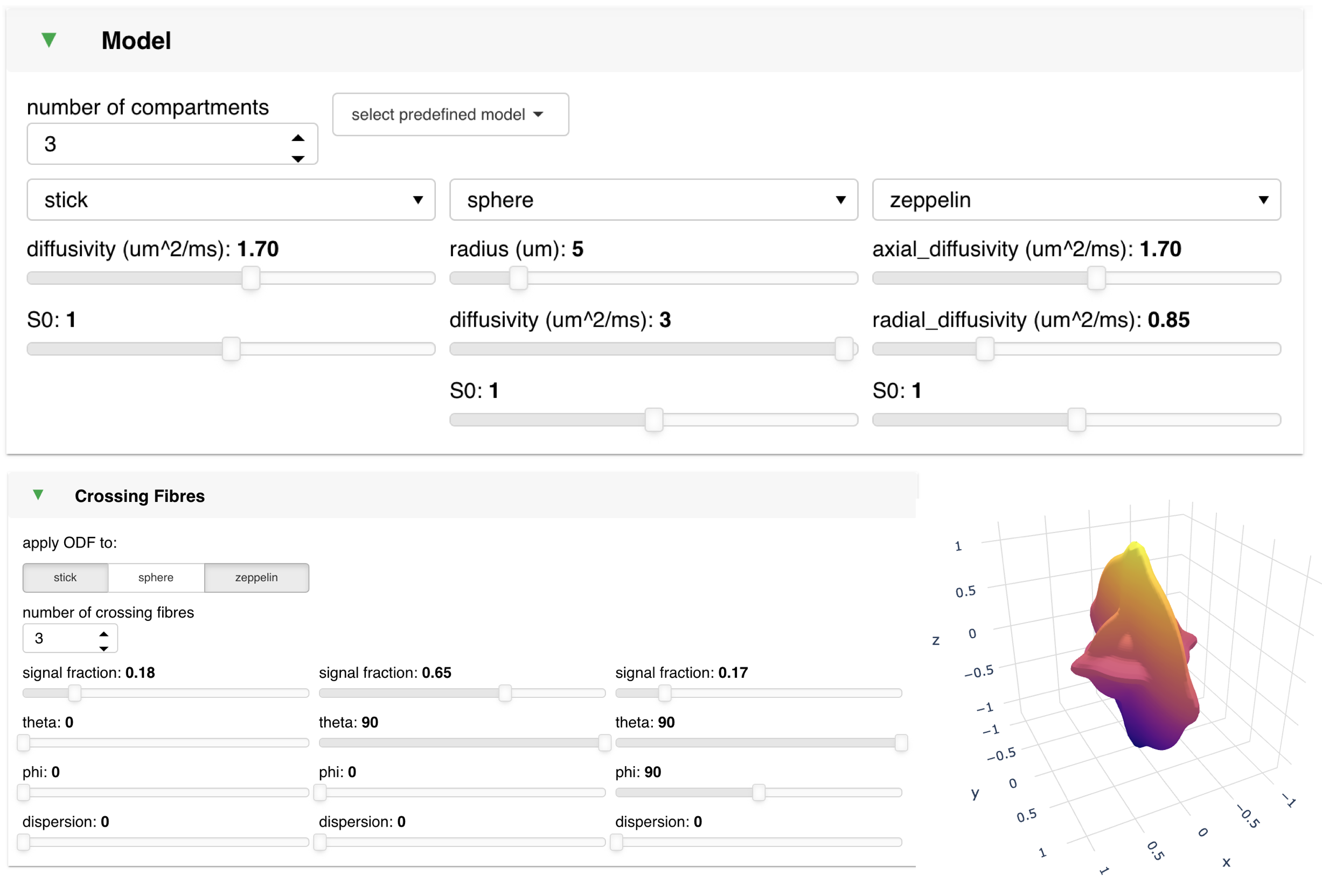
The software is web-based and can be run locally or hosted on a remote web server. The user interacts with the software via the web-browser. It is written in Python and is built upon the Bokeh [4] and Panel [5] libraries for interactive visualisation. The app comprises three components: (a) model specification, (b) acquisition, and (c) visualisation. Figures 1-4 show some of the panels including an example model (SANDI [6]) visualised in various ways.

a. Model specification (Figure 1): the user can specify any number of compartments which are added together to make up the overall signal prediction. In addition to compartments with free or hindered Gaussian diffusion (stick, ball, zeppelin, tensor), we also allow two types of restricted compartments (sphere, to model cell bodies, and cylinder, to model axons), and a compartment for stationary water (dot). The user can also apply an orientation distribution function to all or a subset of the compartments. These are modelled as an arbitrary number of crossing Watson distributions (including stick-like as a special case).

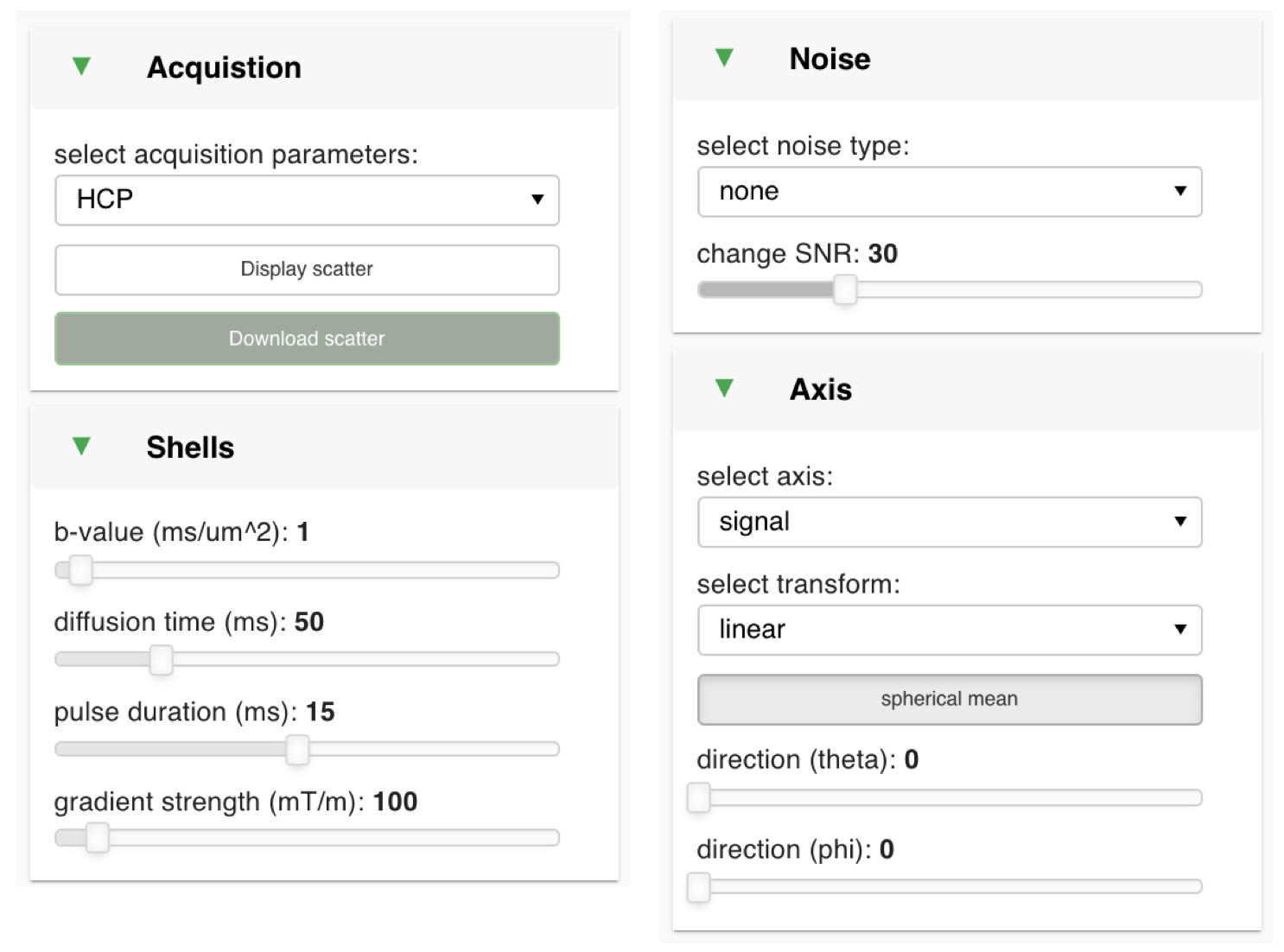
b. Acquisition (Figure 4): currently, the interface assumes a Stejskal-Tanner acquisition [7]. The user can specify a shell (in terms of b-value or its components, i.e., diffusion time, gradient amplitude, and duration). The user can also load a bespoke acquisition protocol and visualise the predicted data under said protocol. Noise can be added to the predictions and the data saved for further analysis (e.g., fitting).

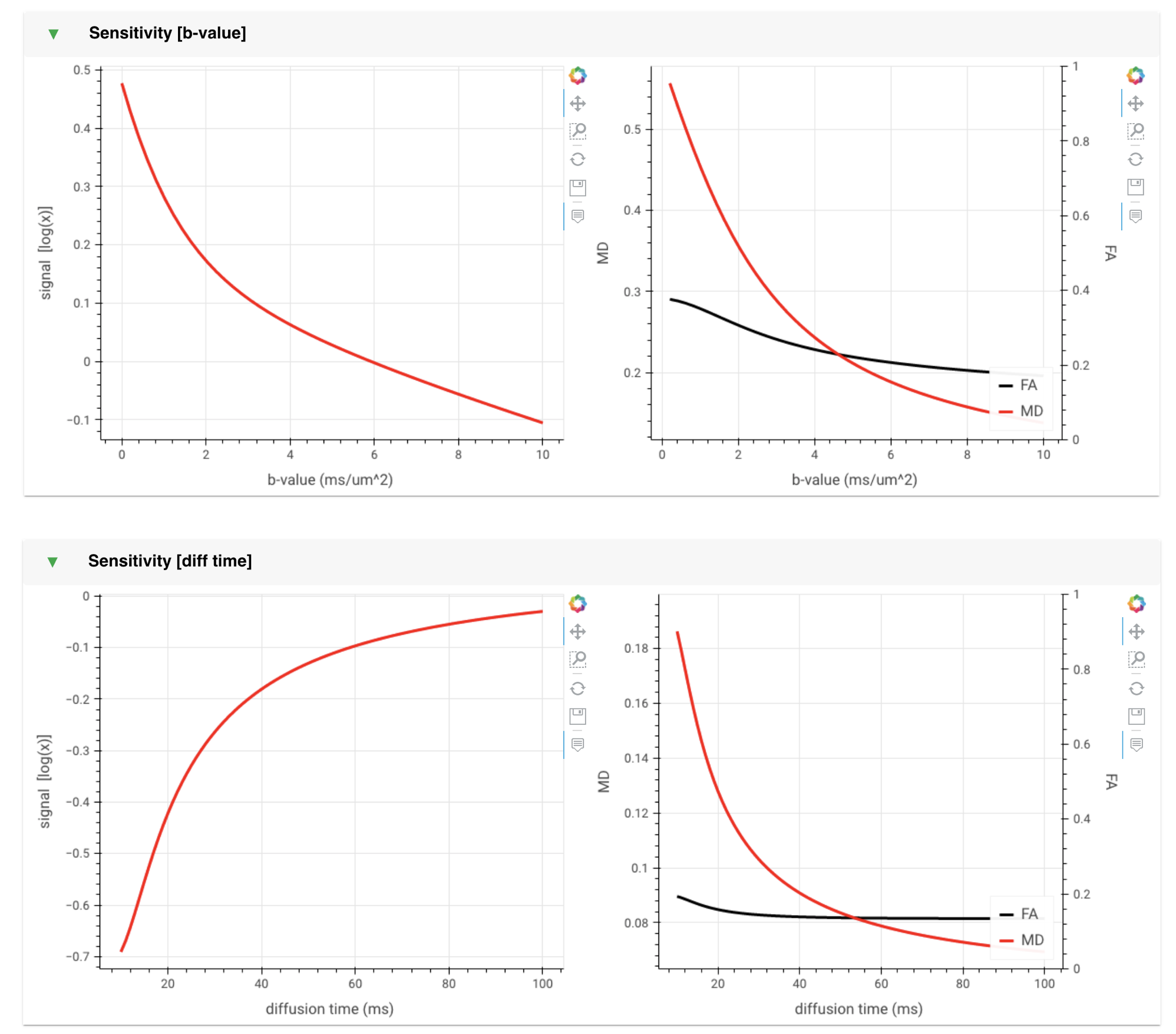
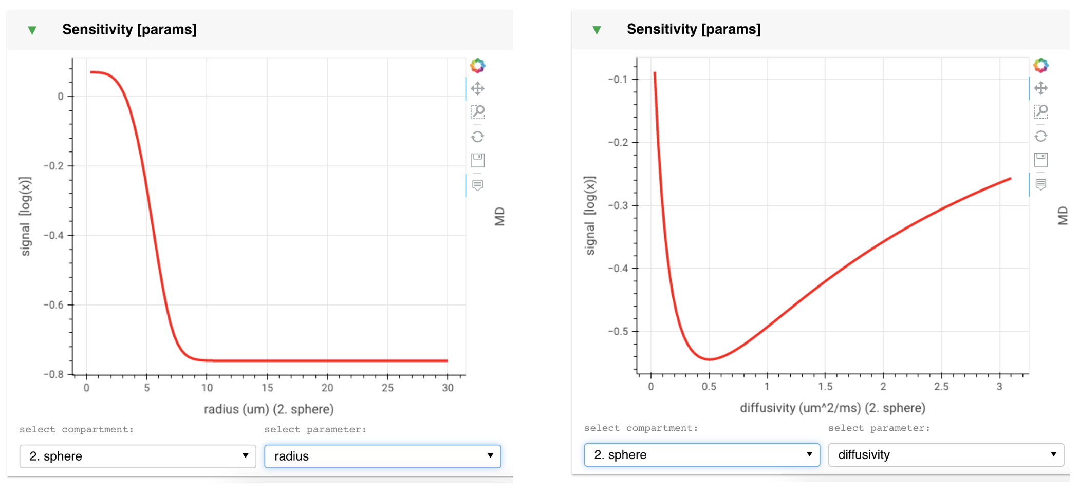
c. Visualisation: multiple panels allow the user to study the model sensitivity to b-value, diffusion time, and gradient orientations (figure 2). There is also a panel for looking at sensitivity to individual model parameters (figure 3). Together, these panels allow a deeper understanding of the model behaviour and limitations.

Future work

There are two immediate improvements to the current framework which are underway, one in the modelling and one in the acquisition. First, we will extend the compartment modelling to allow for exchange between compartments. Second, we will include a more flexible definition of the diffusion acquisition, for example expanding to tensor encoding schemes [8].

Software

https://git.fmrib.ox.ac.uk/fsl/DIVE

See also demo video: https://www.youtube.com/watch?v=9c2-Y1DtbVQ

Acknowledgements

This work is supported by the Wellcome Trust (215573/Z/19/Z and 221933/Z/20/Z). We would like to thank Paul McCarthy (FSLeyes) for his input.

References

[1] F. Sepehrband, D. C. Alexander, N. D. Kurniawan, D. C. Reutens, and Z. Yang, ‘Towards higher sensitivity and stability of axon diameter estimation with diffusion-weighted MRI’, NMR in Biomedicine, vol. 29, no. 3, pp. 293–308, 2016, doi: 10.1002/nbm.3462.

[2] D. S. Novikov, V. G. Kiselev, and S. N. Jespersen, ‘On modeling’, Magnetic Resonance in Medicine, vol. 79, no. 6, pp. 3172–3193, 2018, doi: 10.1002/mrm.27101.

[3] D. S. Novikov, E. Fieremans, S. N. Jespersen, and V. G. Kiselev, ‘Quantifying brain microstructure with diffusion MRI: Theory and parameter estimation’, NMR in Biomedicine, vol. 32, no. 4, p. e3998, 2019, doi: 10.1002/nbm.3998.

[4] Bokeh Development Team, Bokeh: Python library for interactive visualization. 2018. [Online]. Available: https://bokeh.pydata.org/en/latest/

[5] P. Rudiger et al., holoviz/holoviews: Version 1.13.3. Zenodo, 2020. doi: 10.5281/zenodo.3904606.

[6] M. Palombo et al., ‘SANDI: A compartment-based model for non-invasive apparent soma and neurite imaging by diffusion MRI’, NeuroImage, vol. 215, p. 116835, Jul. 2020, doi: 10.1016/j.neuroimage.2020.116835.

[7] E. O. Stejskal and J. E. Tanner, ‘Spin Diffusion Measurements: Spin Echoes in the Presence of a Time‐Dependent Field Gradient’, J. Chem. Phys., vol. 42, no. 1, pp. 288–292, Jan. 1965, doi: 10.1063/1.1695690.

[8] F. Szczepankiewicz, J. Sjölund, F. Ståhlberg, J. Lätt, and M. Nilsson, ‘Tensor-valued diffusion encoding for diffusional variance decomposition (DIVIDE): Technical feasibility in clinical MRI systems’, PLOS ONE, vol. 14, no. 3, p. e0214238, Mar. 2019, doi: 10.1371/journal.pone.0214238.

Figures

Fig 1. Model specification. The user can choose an arbitrary number of compartments amongst: dot, ball, stick, zeppelin, tensor, sphere, and cylinder. Compartment parameters can be changed using slider. Here, the SANDI model has been selected from a list of predefined models. Compartments can be associated with orientation distribution functions, which are modelled as crossings of an arbitrary number of orientations including dispersion. A 3D glyph shows the signal prediction as a function of orientation at a user defined b-value that can also be changed using a slider.

Fig 2. Sensitivity to b-value and diffusion time. The two panels show how the signal depends on the b-value and diffusion time. An additional plot shows how common tensor measures (FA and MD) might change as we change these acquisition parameters. The model simulated here is the one shown in Fig 1 based on the SANDI model. Note that the signal axis is in log-scale, which can be changed by the user to linear scale. Both the b-value and diffusion time axes can also be transformed, e.g. to 1/sqrt(x) or 1/x, which allows the user to visualise different asymptotic behaviours of the model.

Fig 3. Examining parameter sensitivity. The user can visualise the model sensitivity to any changes in the parameters of any compartment. In this example, we see the sensitivity of the powder-averaged signal to the sphere radius on the left, and to the diffusion coefficient of the sphere compartment on the right. Note the non-trivial nonlinear changes in the signal as a function of the diffusion coefficient, which here is due to restricted diffusion.

Fig 4. Acquisition and display controllers. The user can display model predictions for a chosen acquisition. Predictions are displayed as a scatter plot, to which noise can be added with a user-chosen SNR. The data, and relevant acquisition parameters, can be saved as a CSV file for example to feed into a fitting algorithm. The "Shells" panel controls all plots where data is shown at a given b-value, and the "Axis" panel controls the transformations done to various axes, as well as whether the data is powder-averaged (spherical mean) or shown along a specified gradient orientation.

Proc. Intl. Soc. Mag. Reson. Med. 30 (2022)

2692

DOI: https://doi.org/10.58530/2022/2692