2623
What you see is not what you get: localization of Deep Brain Stimulation leads from metal artifacts1Biomedical Engineering, McCormick School of Engineering, Northwestern University, Evanston, IL, United States, 2Radiology, Feinberg School of Medicine, Northwestern University, Chicago, IL, United States, 3Neurosurgery, Feinberg School of Medicine, Northwestern University, Chicago, IL, United States
Synopsis
Deep Brain Stimulation (DBS) implants are implanted into target regions of the brain to treat symptoms of many neurological disorders. Postoperative Magnetic Resonance Imaging (MRI) scans are used to localize DBS leads, however, there are large, distorted artifacts surrounding the leads in the images. This study uses MRI phantoms to investigate the true location of a DBS lead relative to its artifact. The results will help researchers and clinicians know the actual locations of the lead tip and contacts from postoperative MRI scans to confirm the implant is correctly targeting the desired brain area.
Introduction
Deep brain stimulation (DBS) is a powerful neurosurgical tool for treating movement and neurological disorders such as Parkinson’s disease, epilepsy, and dystonia1-3. The procedure involves implanting DBS leads into the brain near a target region that each have multiple metal contacts distributed on the cylindrical leads close to the tip4. Accurate lead localization is crucial for device programming and interpretation of results. Postoperative MRI has grown to be the standard for identifying lead placement, as it accounts for the brain’s natural shifting post-implantation and can be fused with computed tomography (CT) images to improve localization. Metal objects, however, create large distortions on MRI images which makes it difficult to identify the exact position of the lead. Previous research has supported the central position of the lead within the signal void or hypointensity of the lead’s artifact in the plane perpendicular to the lead’s shaft5. However, little is known about the exact location of the lead tip and contacts along the axis of the lead. Intuitively, researchers have assumed that the lead tip is located at the most caudal point of the center of the hypointensity6-8. Here we show that this assumption could cause up to a 2 mm error in lead localization, an error large enough to completely misinterpret DBS small targets.Methods
A skull phantom was designed and 3D-printed from segmented CT images of a DBS patient. A custom holder was also 3D-printed to hold the lead (Abbot/St. Jude Infinity Directional Lead, 6171 model) and four parallel reference marker glass-rods. Each rod was 5 mm away the lead to ensure that the metal artifact did not overlap the image of the rods. The rods in the coronal plane were positioned such that their tip was at the same level of the lead’s tip, whereas the rods in the sagittal plane were positioned at the level of the bottom of the first metallic contact (Figure 1). The holder with lead and reference rods was placed within the skull at an entry point and penetration angle following common DBS surgical practice. The extracranial portion of the lead was looped at the surgical burr hole, similar to our patients. The phantom was placed inside a 20-channel receive-only head/neck coil and scanned at a Siemens 1.5 T Aera scanner using T1MPRAGE and T1TSE sequences with parameters given in Figure 4A. To assess the effects of slice selection and phase encoding direction on the lead’s artifact, each sequence was repeated with different slice selection directions (axial, sagittal, coronal) and with different corresponding phase encoding directions (Anterior-Posterior, Right-Left, Head-Foot, Foot-Head).DICOM images were exported to 3D Slicer in which the artifact around the lead and four rods was manually segmented and used to create triangulated surfaces representing the lead and markers. These 3D masks were then exported to a CAD tool (Rhino 7, Robert McNeal and Associates, Seattle, WA) to be compared against a true non-distorted model of the holder with lead and rods. The true model was manually aligned with the majority of the reference rods in the artifact mask, taking advantage of their minimal distortion (Figure 3A). Once the rods were aligned, the tip of the true lead position was found. The LineThroughtPt function in Rhino was used to create a center line through hypointensity artifact, and then the tip of the line was used as the tip of the artifact. Then we calculated the geometric distance between the tip of the lead’s true point and artifact point.
Results
Changing the acquisition plane and phase encoding direction substantially changed the appearance of the lead’s artifact (Figure 2). The distance between the tip of lead’s artifact from the true tip was 1.812 ± 0.125 mm on T1MPRAGE images and 1.532 ± 0.081 on T1TSE images (Figure 3). A two-tailed t-test for equal variances showed a significant difference between the means (p-value = 0.0009). For both T1MPRAGE and T1TSE sequences, the minimum distance between the true tip and the artifact tip was with the sagittal acquisition plane and A-P phase encoding direction. The maximum distance for these sequences was with the coronal acquisition plane and F-H phase encoding direction. Additionally, in the T1TSE sequences the phase encoding direction affected a clear patterning of alternating hyperintense and hypointense signal regions which can be seen around the four metallic electrode contacts (Figure 2,5).Discussion
There is deviation on the scale of millimeters between the true tip of the lead and the tip of the artifact, therefore the artifact is not indicative of the true lead location along the axis parallel to the lead. Additionally, the amount of variation depends on the type of MRI sequence, acquisition plane, and the phase encoding direction. Lastly, the patterning evident in T1TSE scans can be used to help identify the location of the contacts however the patterning will change depending on the phase encoding direction.Conclusion
A T1TSE MRI image acquired with a sagittal acquisition plane and phase encoding in the anterior-posterior direction (A-P) provides the best images for DBS tip localization. In such case, the true tip of the lead will be about 1.4 mm away from the tip of the void metallic artifact.Acknowledgements
This work was supported by a NIH grant R01EB030324.
References
1. Guridi J and Obeso JA. The subthalamic nucleus, hemiballismus and Parkinson's disease: reappraisal of a neurosurgical dogma. Brain. 2001; 124(1):5-19.2. Fisher R, et al. Electrical stimulation of the anterior nucleus of thalamus for treatment of refractory epilepsy. Epilepsia. 2010; 51(5):899-908.
3. Vidailhet M, et al. Bilateral Deep-Brain Stimulation of the Globus Pallidus in Primary Generalized Dystonia. New England Journal of Medicine. 2005; 352(5):459-467.
4. Lozano AM, et al. Deep brain stimulation: current challenges and future directions. Nature Reviews, Neurology. 2019; 15(3):148.
5. Hyam JA, Akram H, Foltynie T, Limousin P, Hariz M, and Zrinzo L. What you see is what you get: Lead location within deep brain structures is accurately depicted by stereotactic magnetic resonance imaging. Clinical Neurosurgery. 2015; 11(3):412-419.
6. Girgis F, Zarabi. H, Said M, Zhang L, Shahlaie K, and Saez I. Comparison of Intraoperative Computed Tomography Scan with Postoperative Magnetic Resonance Imaging for Determining Deep Brain Stimulation Electrode Coordinates. World Neurosurgery. 2020; 138(e):330-225.
7. Kremer NI, et al. Accuracy of Intraoperative Computed Tomography in Deep Brain Stimulation—A Prospective Noninferiority Study. Neuromodulation: Technology at the Neural Interface. 2019; 22(4):472-477.
8. Bot M, Van Den Munckhof P, Bakay R, Stebbins G, and Verhagen Metman L. Accuracy of intraoperative computed tomography during deep brain stimulation procedures: Comparison with postoperative magnetic resonance imaging. Stereotactic and Functional Neurosurg. 2017; 95(3):183-188.Figures
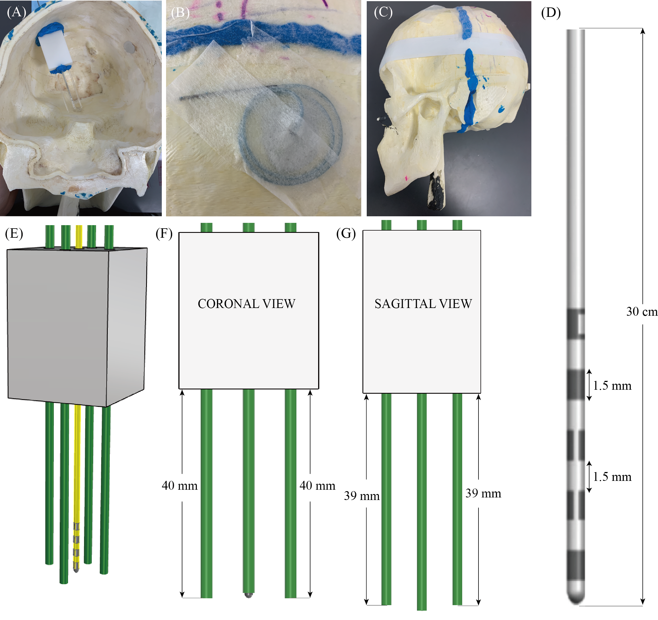
Figure 1: (A) Constructed skull phantom used in experiments with holder, lead, and reference marker rods placed similarly to DBS patients. (B) Extracranial trajectory used for phantom. (C) Completed skull phantom. (D) The Abbot/St. Jude Infinity Directional DBS lead (6171 model). (E) 3D model from Rhino of the holder (grey), lead (yellow), and reference marker rods (green). (F) Coronal plane view of the holder, lead and reference marker rods. (G) Sagittal plane view of the holder, lead, and reference marker rods.
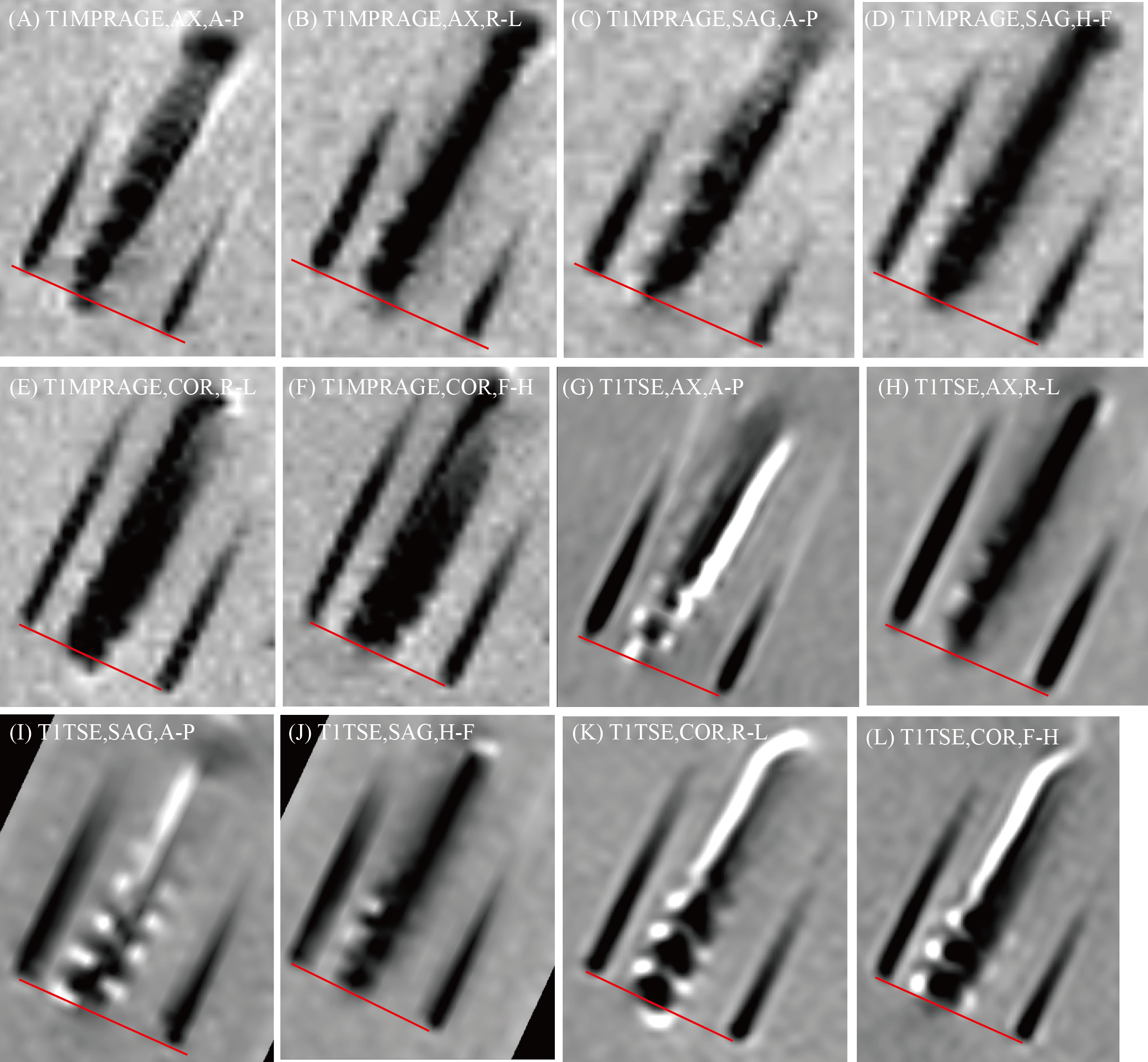
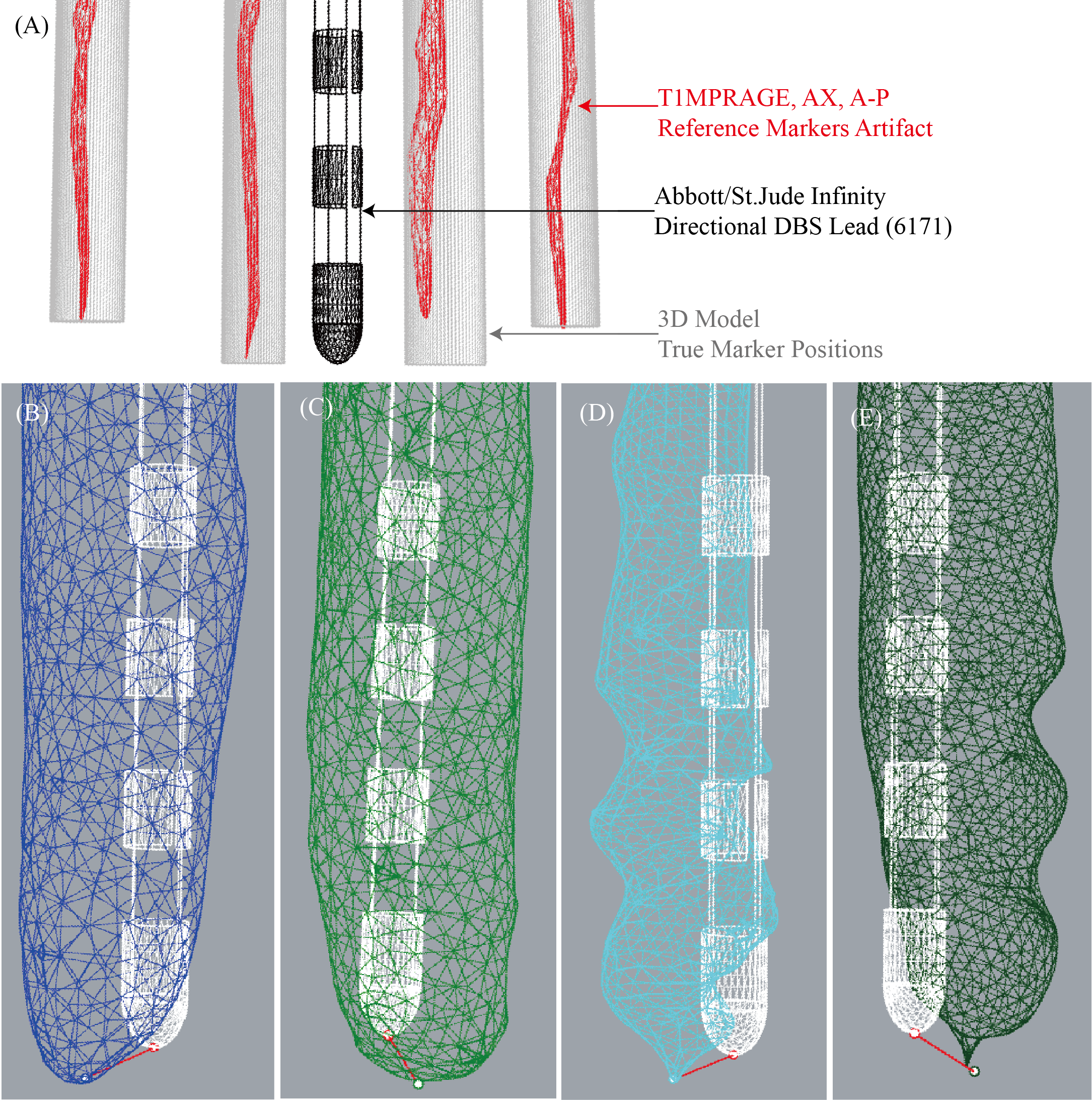
Figure 3: (A) Method for aligning the reference markers’ artifact (red) with the true 3D model of the markers (gray) using the T1MPRAGE, axial, A-P scan as an example. The minimum and maximum distances between the tip of the lead and the tip of the artifact (red lines) for the T1MPRAGE sequence were the (C) Sagittal, A-P, scan and the (D) Coronal, F-H scan, respectively. The minimum and maximum distances between the tip of the lead and the tip of the artifact for the T1TSE sequence were the (E) Sagittal, A-P, scan and the (F) Coronal, F-H scan, respectively.
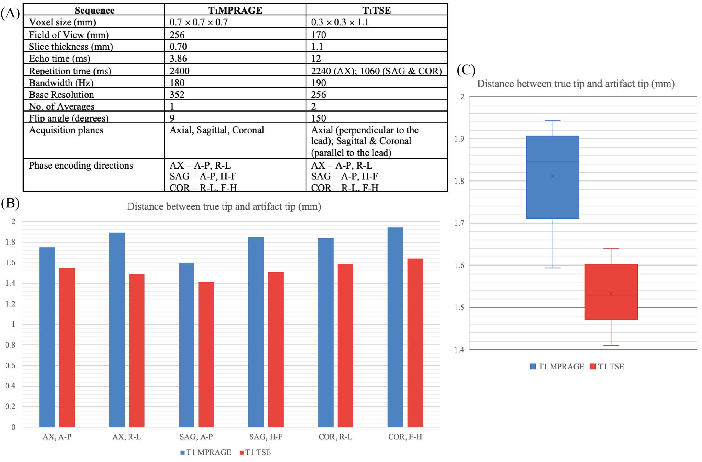
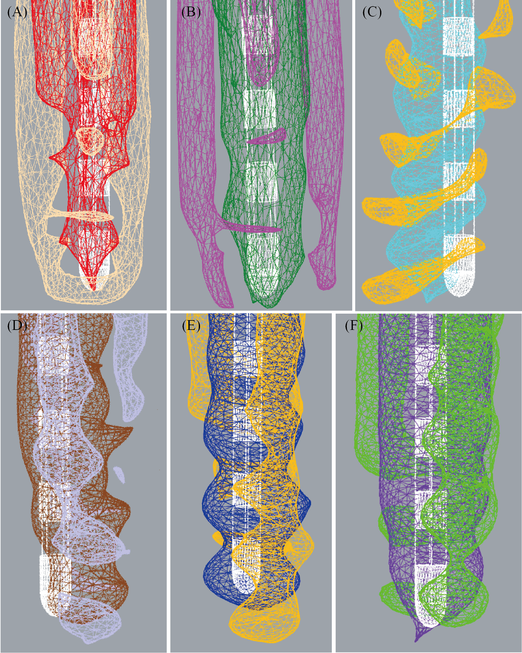
Figure 5: Results from segmenting the hypointense and hyperintense artifacts from the T1TSE scans alongside the true lead position (white) with varying acquisition parameters. (A) Axial, A-P, hypointensity - red, hyperintensity - tan. (B) Axial, R-L, hypointensity - dark green, hyperintensity - magenta. (C) Sagittal, A-P, hypointensity - cyan, hyperintensity - yellow. (D) Sagittal, H-F, hypointensity - brown, hyperintensity - lavender. (E) Coronal, R-L, hypointensity - blue, hyperintensity - orange. (F) Coronal, F-H, hypointensity - purple, hyperintensity - green.