2616
Differences in diffusion-weighted MRS processing and fitting pipelines, and their effect on tissue modeling: Results from a workshop challenge.1C.J. Gorter Center for High-Field MRI, Department of Radiology, Leiden University Medical Center, Leiden, Netherlands, 2Cardiff University Brain Research Imaging Centre (CUBRIC), School of Psychology, Cardiff University, Cardiff, United Kingdom, 3Wellcome Centre for Integrative Neuroimaging, FMRIB, Nuffield Department of Clinical Neurosciences, University of Oxford, Oxford, United Kingdom, 4Center for Magnetic Resonance Research and Department of Radiology, University of Minnesota, Minneapolis, MN, United States, 5Danish Research Centre for Magnetic Resonance, Centre for Functional and Diagnostic Imaging and Research, Copenhagen University Hospital Amager and Hvidovre, Copenhagen, Denmark, 6Magnetic Resonance Methodology, Institute for Diagnostic and Interventional Neuroradiology, University Bern, Bern, Switzerland, 7Translational Imaging Center, sitem-insel, Bern, Switzerland, 8CIBM Center for Biomedical Imaging, Lausanne, Switzerland, 9Animal Imaging and Technology, EPFL, Lausanne, Switzerland, 10LIFMET, EPFL, Lausanne, Switzerland, 11Commissariat à l’Energie Atomique et aux Energies Alternatives (CEA), Centre National de la Recherche Scientifique (CNRS), Molecular Imaging Research Center (MIRCen), Laboratoire des Maladies Neurodégénératives, Université Paris-Saclay, Fontenay-aux-Roses, France, 12Russell H. Morgan Department of Radiology and Radiological Science, The Johns Hopkins University School of Medicine, Baltimore, MD, United States, 13F. M. Kirby Research Center for Functional Brain Imaging, Kennedy Krieger Institute, Baltimore, MD, United States, 14School of Computer Science and Informatics, Cardiff University, Cardiff, United Kingdom
Synopsis
A processing and fitting challenge was initiated for the “Best practices & Tools for Diffusion MR Spectroscopy” workshop held at the Lorentz Center (Leiden, NL) in September 2021. Our goal was to assess variabilities in processing and fitting pipelines and possibly identify the most robust steps to analyze diffusion-weighted MRS data. A “brain-like” dataset of diffusion-weighted spectra was simulated and participants were asked to analyze the data with their routinely used pipelines. Results showed that variabilities between participants (n=8) particularly increased at higher b-values and for J-coupled metabolites (Ins, Glu) as a result of lower SNR and higher CRLB values.
Introduction
Diffusion-weighted MR spectroscopy (DWMRS) is a unique tool to non-invasively probe the microstructure of cell-specific intracellular spaces in vivo[1]. Indeed, DWMRS has the potential to serve as a biomarker for neurodegeneration (neuronal-markers: tNAA, Glu) and neuroinflammation (astrocytic/glial-markers: tCho, Ins)[2,3,4], where processing and fitting of DWMRS data significantly impacts the estimation of metabolites’ diffusion properties and, in turn, accurate modeling of cell-specific microstructural features. Although most processing and fitting steps overlap with methods used for standard MRS[5], DWMRS also relies on the evaluation of multiple spectra acquired under different conditions (e.g. various b-values, encoding directions, etc.). Data at higher b-values are more prone to error, due to: higher sensitivity to motion, stronger individual phase drift, and lower SNR.As the DWMRS community grows, we wanted to investigate how reproducible and reliable our research is, and possibly identify the most robust steps to process and fit DWMRS data. This was the aim of a workshop held at the Lorentz center in Leiden (NL) in September 2021. During the workshop, a processing and fitting challenge was proposed to the participants. We hereby present the setup of the challenge and its main results.
Materials & Methods
Deposited dataset: Simulated spectra of brain metabolites were generated using Matlab for a STEAM sequence with TE/TM=45/60ms at 7T (ideal RF-pulses, spectral width 3 kHz, 1024 complex points), and relying on published chemical shifts, J-coupling constants[6], metabolite concentrations and T2 relaxation values[7]. A synthetic spectrum consisted of a weighted sum of 17 metabolites and included a macromolecular (MM) baseline (Fig.1A). Signal attenuation for individual metabolites at 9 different b-values (ranging from 0 to 50 ms/μm2) was generated using a model based on randomly oriented infinite cylinders[8] and a mono-exponential decay for the MM (Fig.1B), resulting in 9 diffusion-weighted synthetic spectra (Fig.1C). Finally, to emulate in-vivo datasets, a total of 32 transients for each diffusion-weighting condition were imposed with independent line-broadening, random complex Gaussian noise, and frequency and phase drift (Fig.1D/E). The range for frequency drift across transients was similar for all b-values ([-4,4] Hz), but phase drift was increased with b-value. Ground-truth (GT) spectra (without noise and drifts) and synthetic spectra (with noise/frequency/phase drifts), sequence details, and a basis-set for fitting were shared on GitHub (https://github.com/dwmrshub/pregame-workshop-2021). The model used to generate signal attenuation across b-values and the GT on individual frequency and phase drifts were not shared with participants.Challenge deliverables: The processing and fitting steps submitted by each participant (n=8) are summarized in Fig.2. To disentangle the effect of processing and fitting steps, we asked for the following deliverables:
(1) Processing alone: residuals between the GT and processed spectra at each b-value (Fig.3A) and the phase/frequency corrections applied at each transient.
(2) Fitting alone: signal decays (normalized to b=0ms/μm2) of 5 metabolites (tNAA, tCr, tCho, Glu, and Ins) and MM for the GT data. Not shown.
(3) Processing+fitting: signal decays (normalized to b=0ms/μm2) of 5 metabolites and MM for the processed and fitted synthetic spectra (Fig.3B).
Modeling: The original model (Fig.1B) was applied to the signal decays generated from the processed and fitted synthetic spectra to evaluate how much variability in the spectral fit affects the estimation of biophysical parameters (Fig.4C). Apparent diffusion coefficients (ADCs) were also computed with a mono-exponential fit applied between b=0 and b=3ms/μm2 (Fig.4B).
Results & Discussion
As reported in Fig.2, participants used different platforms to process and fit the DWMRS data. All pipelines included individual phase-and-frequency correction. The various processing pipelines resulted in differences in residuals between processed spectra and GT (Fig.3), illustrating pipeline-specific peculiarities. This can also be appreciated from the difference in MSE between the fitted GT and synthetic data (Fig.3B). Fig.3C shows variability across participants due to both processing and fitting steps. Decays are relatively similar for tNAA and tCr and slightly more variable for tCho at higher b-values. Results for J-coupled metabolites and MM are more variable across b-values due to lower SNR and increased CRLBs at higher b-values (Fig.4). Such differences could potentially be alleviated by acquiring more transients at higher b-values. ADCs given in Fig.4A, and Fig.4C illustrate the variability in the modeling output (radii and Dintra).Conclusion
This processing and fitting challenge is a first step towards understanding points of convergence and divergence in different processing and fitting pipelines. Most participants were already very familiar with DWMRS and yet results substantially vary as soon as conditions worsen (typically when CRLBs > ~5%). Further analyses will account for the fitting variability (typically, using the CRLBs) to report this uncertainty on the modeling. Dynamic fitting approaches (e.g. P1 and P7) fitting the spectra including a prior about the expected decay (here, bi-exponential) could help reduce the uncertainty at high b-values. The challenge is still open to everyone interested in DWMRS. Future steps will include recruiting more participants, and more realistic distorsions to match in-vivo conditions (eddy-currents, lineshape, amplitude variation, SNR, etc.).Acknowledgements
This abstract was initiated by the Workshop ‘Best Practices & Tools for Diffusion MR Spectroscopy’, held at the Lorentz Center, Leiden, The Netherlands on 20-24 September 2021, and tremendously benefited from committed discussions among the attendees. The workshop has received funding from the Lorentz center and NeurATRIS (A Translational Research Infrastructure for Biotherapies in Neurosciences, “Investissements d'Avenir”, ANR-11-INBS-0011). HL and NJ have received funding from the European Research Council (ERC) under the European Union’s Horizon 2020 research and innovation programme (grant agreement No 804746). AD received funding from the Swiss National Science Foundation (SNSF #188142, #202962). GG received funding from the National Institutes of Health [grant numbers R01MH113700, R01AG039396, P41 EB015894, P30 NS076408] and the W.M. Keck FoundationReferences
[1] Palombo, Shemesh, Ronen, Valette, NeuroImage 2018
[2] Ercan et al., Brain 2016
[3] Ligneul et al., NeuroImage 2019
[4] Genovese et al., NMR in Biomed 2021
[5] Near et al., NMR in Biomed 2021 (experts consensus)
[6] Govindaraju, NMR in Biomed, 2000
[7] Marjanska, NMR in biomedicine, 2012
[8] Balinov, J. Magn. Reson., 1993
[9] Veraart et al., MRM, 2016
[10] Jelescu et al., ISMRM, 2020
[11] Simpson et al., MRM, 2017
[12] Clarke et al., MRM, 2020
[13] Oeltzschner et al., J. Neurosci. Methods (JNMEDT), 2020
[14] Adalid et al., MAGMA, 2017
[15] Provencher. NMR Biomed, 2001
Figures
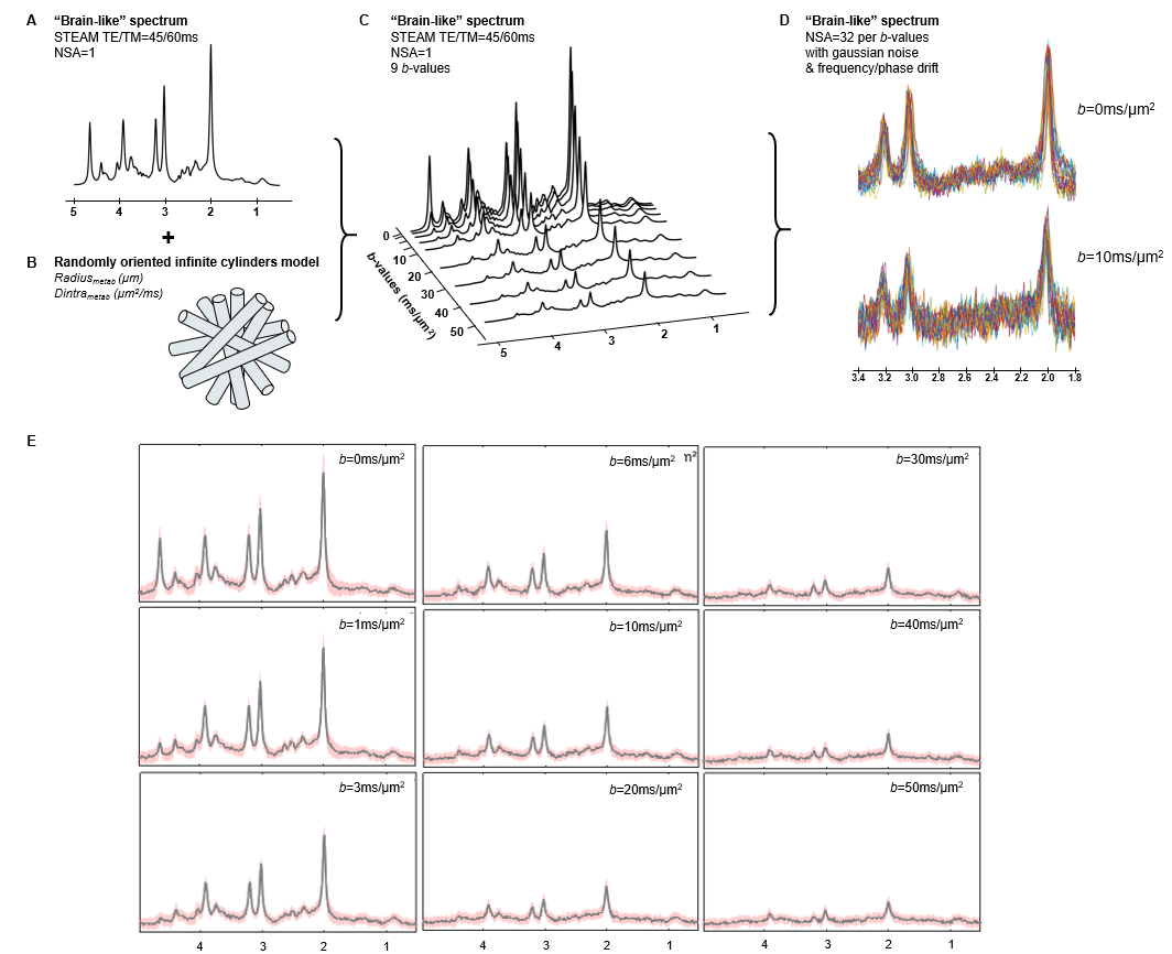
Figure 1
(A) A “brain-like” spectrum was generated.
(B) Signal decay was generated using a randomly oriented infinite cylinders model, (specific radius and intracellular free diffusivity (Dintra) for each metabolite).
(C) Diffusion-weighted spectra were generated for 9 b-values
(D) 32 transients were created for each b-value using random noise, frequency and phase drift across transients.
(E) Illustration of the signal at each b-value (shaded red area: fluctuations in frequency/phase across transients; black line: average).
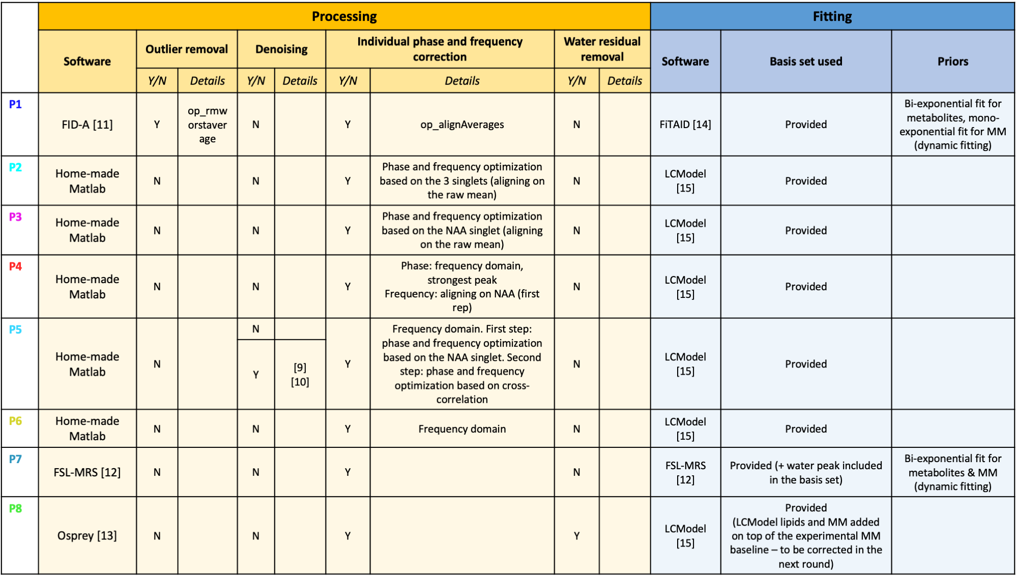
Figure 2
Table summarizing the processing and fitting steps for each participant.

Figure 3
Results from the processing and fitting challenge.
(A) Residuals from the processing step (range ~1.5-4.0 ppm): the processed spectra were subtracted from the ground truth spectra (Fig.1C).
(B) Signal decays of 5 metabolites + MM for each participant. The black line corresponds to the ground truth signal decay.
(C) Mean squared errors (MSEs) of signal decays reported in (B) for each participant. MSEs are given for each metabolite and averaged in the last column.
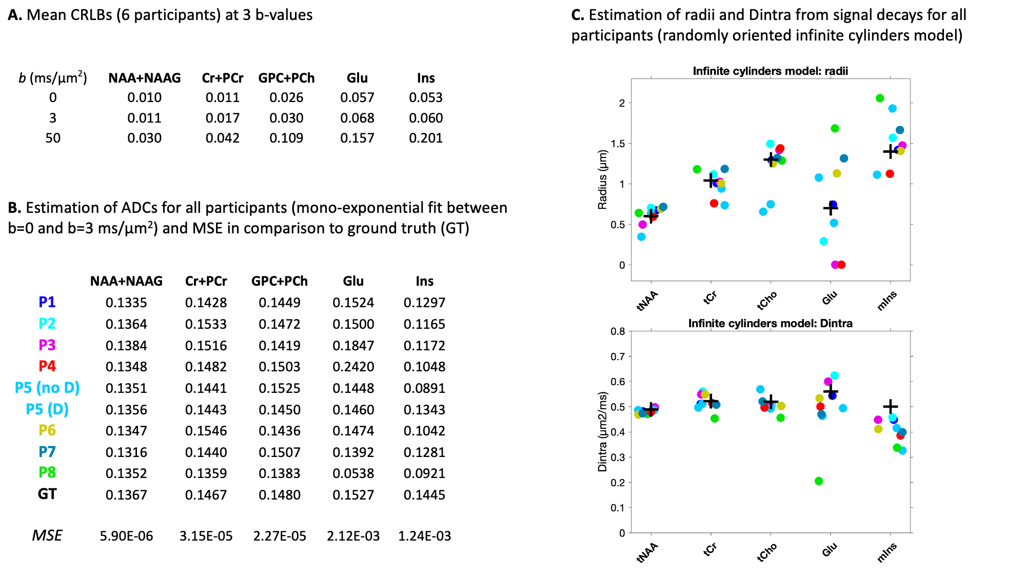
Figure 4
(A) Mean relative CRLBs at 3 b-values
(B) Estimation of ADCs for all participants and the ground truth (GT). A mono-exponential fit was applied to the signal decay between b=0 and b=3 ms/µm2
(C) Estimation of radii and Dintra for all participants (2 methods for P5). The black cross corresponds to the GT. A randomly oriented infinite cylinders model was applied to the signal attenuations reported in Fig.3C.