2606
Comparison of machine learning methods for detection of prostate cancer using bpMRI radiomics features
Ethan J Ulrich1, Jasser Dhaouadi1, Robben Schat2, Benjamin Spilseth2, and Randall Jones1
1Bot Image, Omaha, NE, United States, 2Radiology, University of Minnesota, Minneapolis, MN, United States
1Bot Image, Omaha, NE, United States, 2Radiology, University of Minnesota, Minneapolis, MN, United States
Synopsis
Multiple prostate cancer detection AI models—including random forest, neural network, XGBoost, and a novel boosted parallel random forest (bpRF)—are trained and tested using radiomics features from 958 bi-parametric MRI (bpMRI) studies from 5 different MRI platforms. After data preprocessing—consisting of prostate segmentation, registration, and intensity normalization—radiomic features are extracted from the images at the pixel level. The AI models are evaluated using 5-fold cross-validation for their ability to detect and classify cancerous prostate lesions. The free-response ROC (FROC) analysis demonstrates the superior performance of the bpRF model at detecting prostate cancer and reducing false positives.
Introduction
The purpose of this work was to develop an improved computer-aided diagnostic model for predicting prostate cancer from radiomics features extracted from prostate bi-parametric MR images (bpMRI).Methods
A database of 958 prostate bpMRI scans from three MRI scanner manufacturers (GE: 111, Philips: 655, Siemens: 192) and included 521 1.5T and 437 3.0T cases from a public source1-3 and six participating research partners. These cases represent a sample of the general population of men (median age 66 years; range 37-90 years) referred for prostate MRI and included bpMRI series following PI-RADS4 acquisition recommendations. Annotations for cancer (Gleason grade ≥ 7), benign (including Gleason 6), and normal tissues were created using 3D targeted biopsy locations and clinical reports provided by the contributing sources.MRI study prostate volumes were preprocessed by registering the ADC and the highest b-value DWI (median 1400 s/mm2; range 600-2000 s/mm2) to the axial T2w volume to improve alignment. The axial field-of-view was standardized to be 140 mm centered on the prostate. T2w intensities were normalized using NU normalization5 with ten landmarks to standardize the intensity probability density function. High b-value DWI volumes were normalized using a min-max scaler on intensities within the prostate. ADC intensities were truncated to be between 0 and 2500 mm2/s.
A total of 64 radiomics features were extracted following the method of Lay6, which consisted of intensity and texture features from the preprocessed T2w, DWI, and ADC image slices. Four pixel-wise cancer prediction models were trained: a neural network (NN), a model based on XGBoost7 (XG), a traditional random forest8 (RF) model with fixed instance weighting following the work of Lay6, and an ensemble boosted parallel random forest (bpRF) model with boosting by AdaBoost9.
The proposed bpRF model (Figure 1) starts by fitting a bagging estimator10 of five parallel random forest classifiers on the original dataset. For each boosting iteration, the bagging estimator generates five data subsets by randomly subsampling 50% of both samples and features from the original dataset and feeds each of the parallel random forests with one of them. At the end of each boosting iteration and by implementing its AdaBoost component, the bpRF model interprets the average prediction of the bagging estimator—which is based on the individual predictions of the five parallel random forests—and adjusts weights for incorrectly classified instances. Hence, the subsequent bagging estimators focus more on difficult cases and learn how to avoid previous misclassifications.
All models were trained and evaluated using five-fold cross-validation and results were compared using ROC and free-response ROC (FROC) analyses. Folds were generated by dividing the dataset into 5 homogeneous groups. Stratified sampling was performed to preserve ratios of the subject characteristics (i.e., biopsy outcome, scanner manufacturer, field strength). Pixel-level sampling was then performed on each study to maintain a class balance between cancerous and noncancerous pixel samples within each fold. ROC analysis evaluated model predictions at each biopsy location and compared them to the pathology outcomes. The prediction value at each biopsy location was determined using a Gaussian-weighted function centered at the biopsy point. This method assigns higher weights to predictions near the center of the biopsied region and accounts for the uncertainty of the exact biopsy location. Additional detections were defined as local maxima that occur more than 6 mm away from a known lesion—these classified as false positives. The prediction value at each additional detection was determined using the same weighted function as was used for the biopsy point predictions.
Results
Figure 2 depicts ROC analysis results. The NN model had significantly lower AUC when compared to bpRF (p=0.004) and XG (p=0.046) after adjusting for multiple comparisons. Figure 3 depicts FROC analysis results. The performance metric for FROC is the weighted alternative FROC (wAFROC) figure of merit11 and is analogous to the ROC AUC. The bpRF model had significantly higher performance when compared to NN (p=0.007), RF (p=0.003), and XG (p=0.002) after adjusting for multiple comparisons. Figures 4 and 5 illustrate examples of bpMRI image sets processed by the various models compared to expert radiological segmentation of tumors (yellow outline).Discussion
While all models demonstrated similar performance when evaluating at the lesion-level (ROC analysis), bpRF outperforms other models on FROC analysis. This indicates that the bpRF model produced fewer false positive detections at equal sensitivity. Note that the ROC analysis was a harsh evaluation because biopsies were only taken from suspect tissue, hence, no credit was received to properly classify “easy” normal tissue. Another limitation is that the ROC analysis does not account for false positives outside the lesions that were biopsied. FROC analysis overcomes these limitations by evaluating model predictions at each biopsy location and additional detections in the regions of normal tissue. A comparison of detection performance between the CAD method and the average reader, and effect on radiologist reader outcome, is beyond the scope of this paper and will be the subject of future work.Conclusion
A boosted parallel random forest model with T2w, DWI, and ADC intensity and texture features for detecting prostate cancer outperforms other machine learning methods and has the potential to improve physician performance interpreting prostate MRI.Acknowledgements
No acknowledgement found.References
- Litjens G, Debats O, Barentsz JO, Karssemeijer N, Huisman H. Computer-aided detection of prostate cancer in MRI. IEEE Trans Med Imaging. 2014;33(5):1083-1092.
- Litjens G, Debats O, Barentsz JO, Karssemeijer N, Huisman H. ProstateX Challenge data, The Cancer Imaging Archive. 2017.
- Clark K, Vendt B, Smith K, et al. The Cancer Imaging Archive (TCIA): maintaining and operating a public information repository. J Digit Imaging. 2013;26(6):1045-1057.
- Turkbey B, Rosenkrantz AB, Haider MA, et al. Prostate imaging reporting and data system version 2.1: 2019 update of prostate imaging reporting and data system version 2. Eur Urol. 2019;76(3):340-351.
- Nyul LG, Udupa JK. Standardizing the MR image intensity scales: making MR intensities have tissue-specific meaning. In Medical Imaging 2000: Image Display and Visualization. 2000;3976:496-504.
- Lay NS, Tsehay Y, Greer MD, et al. Detection of prostate cancer in multiparametric MRI using random forest with instance weighting. J Med Imaging. 2017;4(2):024506.
- Friedman JH. Greedy function approximation: a gradient boosting machine. Annals of Statistics. 2001;1189-1232.
- Breiman L. Random forests. Machine Learning. 2001;45(1):5-32.
- Freund Y, Schapire RE. A decision-theoretic generalization of on-line learning and an application to boosting. J Computer and System Sciences. 1997;55(1):119-139.
- Breiman L. Bagging predictors. Machine Learning. 1996;24(2):123-140.
- Chakraborty DP, Zhai X. On the meaning of the weighted alternative free‐response operating characteristic figure of merit. Med Phys. 2016;43(5):2548-2557.
Figures
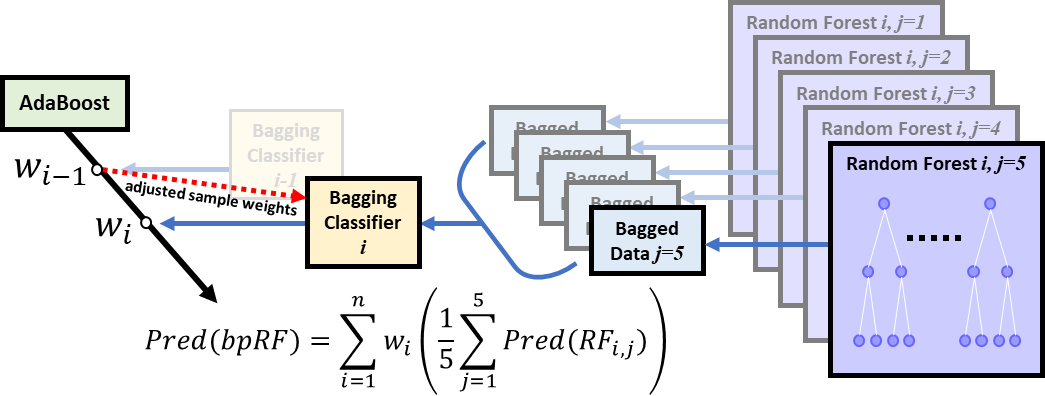
Figure 1: The proposed boosted parallel random forest (bpRF)
model architecture. bpRF is an ensemble of various base models. The
ensemble model seeks the wisdom of the crowd and aggregates the
prediction of each base model to make a final prediction
with less generalization error. bpRF implements a chain of estimators
that starts with an AdaBoost model encapsulating multiple bagging
classifiers that are boosted sequentially during training. Each
bagging classifier has 5 parallel random forests acting on random
slices of data.
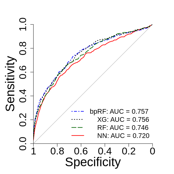
Figure 2: Lesion-level
ROC analysis of the four prostate cancer prediction models.
Predictions are evaluated at each biopsy location, with positives
defined as biopsy results with combined Gleason score ≥ 7. Curves
and AUCs are the average of the cross-validation folds. All
prediction models have similar performance when evaluating
exclusively at the biopsy point locations. NN = neural net, XG =
XGBoost, RF = random forest, bpRF = boosted parallel random forest.
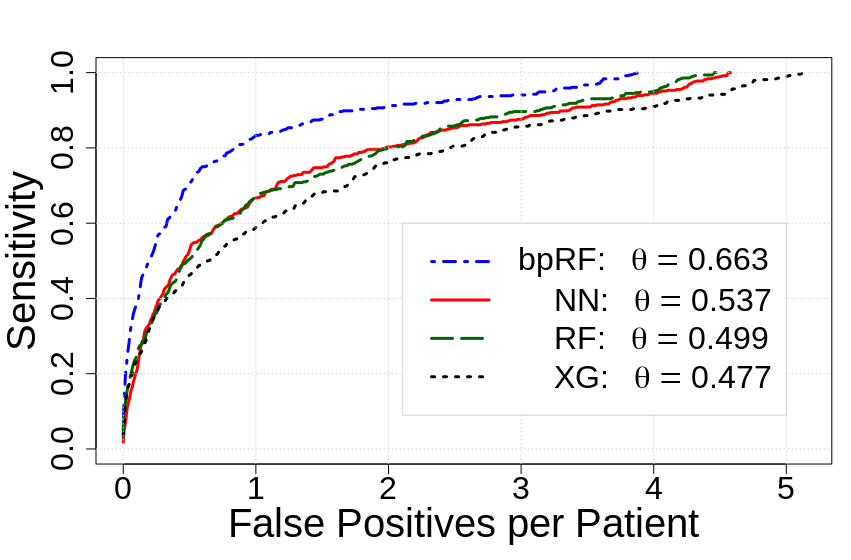
Figure 3: Free-response
ROC (FROC) analysis of the four prostate cancer prediction models.
Detections are evaluated at each biopsy location and local maxima
within the predicted probability map. False positives are defined as
detections at biopsy sites with combined Gleason score < 7 or a
local maximum that is more than 6 mm from a known lesion. Curves and
the performance metric (θ) are the average of the cross-validation
folds. NN = neural net, XG = XGBoost, RF = random forest, bpRF =
boosted parallel random forest.
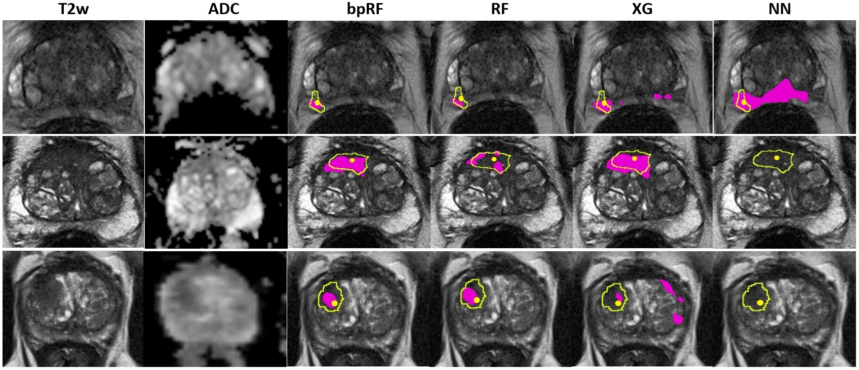
Figure 4:
Model predictions (pink) on prostates with cancer.
Yellow outlines are lesion boundaries drawn by experts
following PI-RADS v2.14. Outside pink regions reflect false positive predictions. Yellow dots indicate biopsy locations. Top: subject with small cancerous lesion in the right
posterior PZ. Center: subject with large cancerous lesion in the
anterior TZ to the right of midline. Bottom: Subject with cancerous lesion in the right anterior TZ. NN = neural net, XG =
XGBoost, RF = random forest, bpRF = boosted parallel random forest,
PZ = peripheral zone, TZ = transition zone.
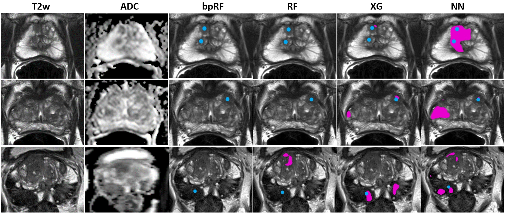
Figure 5: Model predictions (pink) on prostates with benign lesions, hence, all pink regions reflect false positive predictions.
Biopsy locations are indicated by a blue dot. Top:
subject with benign lesions in the right anterior PZ and the
right mid TZ. Center: subject with a small benign lesion in the left
anterior TZ. Bottom: subject with large benign lesions in the posterior PZ
(only one biopsy location is visible in the slice shown). NN = neural
net, XG = XGBoost, RF = random forest, bpRF = boosted parallel random forest,
PZ = peripheral zone, TZ = transition zone.
DOI: https://doi.org/10.58530/2022/2606