INTRODUCTION

Up to 80% of patients who present with cardiac arrest to U.S. hospitals are comatose after the return of spontaneous circulation (ROSC)¹. Although targeted temperature management (TTM) has improved the outcome in patients resuscitated after cardiac arrest, approximately 45-70% of these patients still die or have a poor neurological outcome at hospital discharge², and 50% of survivors have long-term neurocognitive deficits³. A better characterization of the mechanism of ongoing brain injury is required to develop and assess new treatments.
Magnetic resonance spectroscopy has been to be highly sensitive to changes in the brain after TTM after cardiac arrest namely showing significant reductions in N-acetylaspartate (NAA), a neuronal marker, and lactate (Lac), a marker of hypoxia⁴. Initial findings show that a lactate/creatine ratio above 0.23 would prognose poor outcome with good sensitivity and specificity, however, if all metabolites could be utilized, a much greater accuracy could be achieved. Our goal in this study is to apply machine learning methods such as z-scores, decision-tree modeling, principal component analysis, and linear support vector machine to provide a metabolic signature for outcomes after TTM in cardiac arrest.

METHODS

Dataset: This study includes n=39 patients who underwent TTM for coma after cardiac arrest and ROSC at the Brigham and Women's Hospital. The clinical outcome was defined as "good" if the patient regained the ability to open their eyes and follow verbal commands before hospital discharge; any less response is considered as a "poor" outcome⁴. Inclusion criteria for control subjects n=25 were healthy athletic male volunteers without a history of neurological disease. Our data analysis includes subjects who underwent proton MRS on a 3T MRI (Siemens TIM Verio) using a 32 channel head coil using short-echo-point-resolved (PRESS) single voxel spectroscopy (TE=30ms, TR=2s, 128 averages, 8 cc volume) in the posterior cingulate of the brain.
Quantification: The single-voxel MRS raw data were pre-processed using Suspect library⁵. Pre-processing includes channel combination, frequency drift correction, residual water suppression, and/or eddy-current correction. The pre-processed spectra were quantified using LCModel⁶. Concentration of the following metabolites are used in our data analysis: total NAA (tNAA, including NAA + NAA-Glutamate), total creatine (tCr, including Creatine + PhosphoCreatine), total Choline (tCho, including PhosphoCholine + Choline), Glutamate (Glu), Glutamine (Gln), myoinositol (Ins), Glutathione (GSH), Lactate (Lac) and GABA. In all subjects, the Cramer-Rao Lower Bounds (CRLB) for tNAA, tCr, tCho, and Ins was less than 20%, and the subjects with low Lac were included in the analysis to avoid any study bias.
Data Analysis: The data analysis pipeline is shown in Figure 1. First, for the control data, we compute CRLB (%SD)-based weighted average and standard deviation for the metabolites using the following equations for metabolites with CRLB (%SD) < 999 and the unweighted average for metabolites with CRLB (%SD) = 999.
$$$\overline{C} = \sum{w}_{j}{C}_{j}/\sum{w}_{j}, {w}_{j} = 1/{\sigma}_{j}, {\sigma}_{j}= {(\%S.D)}_{j}{C}_{j}/100$$$
$$$\sigma(\overline{C}) = 1/\sqrt{\sum{w}_{j}}$$$
The weighted average and standard deviation values are used in z-score computation for the control data using equation $$$z = ({C}_{j} - \overline{C})/\sigma(\overline{C})$$$.
To compute the z-score for patient data, we use the control data's weighted average and standard deviation. This process enhances the differences between the control and patient data. Next, we use the decision tree model to fit and visualize the z-score data to determine metabolite threshold to differentiate among controls, poor-outcome, and good-outcome. Finally, we perform principal component analysis (PCA) and determine the principal components that enable the identification of potential biomarkers. Finally, we use a linear support vector machine model to visualize the decision boundary of the principal components.

RESULTS and DISCUSSION

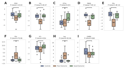
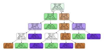
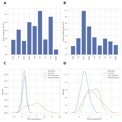
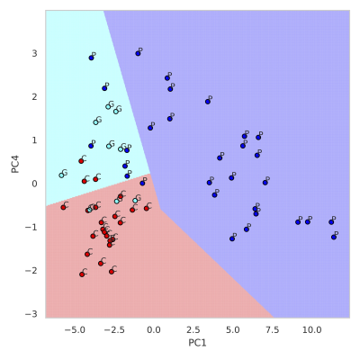
Figure 2 summarizes the z-score analysis and shows the ANOVA-based p-value for each metabolite. As observed in previous studies⁴ tNAA, concentration is high for controls and good-outcome subjects compared to poor-outcome subjects and Lac shows the opposite trend. We observe that multiple metabolites show significance, however, the order of importance of the metabolites is unknown. We use the decision tree in Figure 3 to visualize the interaction among metabolites and the order of importance of the metabolites. For example, the path from tNAA->tCho->Lac suggests the threshold for identifying good and poor outcome patients. We performed PCA to determine the contribution of each metabolite to differentiate among controls, good-outcome, and poor-outcome categories. PCA analysis generated nine principal components (PCs) from the nine metabolites. We apply ANOVA analysis to these nine PCs to determine PCs that separate the three categories statistically. Figures 4A-B show the factor loading for the two chosen PCs, and Figure 4C-D their corresponding kernel density estimation. PC1 separates control and good-outcome data from poor-outcome data, and PC4 separates control from patient data. PC1 and PC4 are used in the linear support vector machine model to generate the decision boundary in Figure 5. The weighted F1 score of the model is 0.80 and it shows a clear separation among the three categories.

CONCLUSION

This work presented an interpretable machine learning-based pipeline to systematically identify the metabolic signatures. It is evident from the analysis that changes to the concentration of tNAA, and Lac has a significant effect on the outcome of the patient, as in previous⁴. Additionally, tCho, Gln, Ins, and GSH have a significant contribution towards the patient outcome.

Acknowledgements

No acknowledgement found.

References

1. Holzer M. Targeted temperature management for comatose survivors of cardiac arrest. N Engl J Med. 2010;363(13):1256-64.

2. Bernard SA, Gray TW, Buist MD, Jones BM, Silvester W, Gutteridge G, Smith K. Treatment of comatose survivors of out-of-hospital cardiac arrest with induced hypothermia. N Engl J Med. 2002;346(8):557-63.

3. Steinbusch CVM, van Heugten CM, Rasquin SMC, Verbunt JA, Moulaert VRM. Cognitive impairments and subjective cognitive complaints after survival of cardiac arrest: A prospective longitudinal cohort study. Resuscitation. 2017;120:132-7.

4. Lee JW, Sreepada L, Bevers M, Li K, Scirica B, da Silva DS, Henderson GV, Bay C, Lin AP. Magnetic resonance spectroscopy of anoxic brain injury after cardiac arrest. medRxiv. 2021.

5. Rowland, B.C., Sreepada, L.P., Jiang, S.H., & Lin, A.P. (2017). OpenMRSLab: An open‐source software repository for magnetic resonance spectroscopy data analysis tools.

6. Provencher, S. (2020) LCModel and LCMgui User’s Manual. http://s-provencher.com/pub/LCModel/manual/manual.pdf