2599
Accuracy and repeatability of joint sparsity multi-component estimations in MR Fingerprinting1Imaging Physics, Delft University of Technology, Delft, Netherlands, 2Department of Radiology and Nuclear Medicine, Erasmus MC, Rotterdam, Netherlands, 3Department of Radiology, Leiden University Medical Centre, Leiden, Netherlands, 4C.J. Gorter Center for High Field MRI, Radiology Department, Leiden University Medical Centre, Leiden, Netherlands
Synopsis
Multi-component MR Fingerprinting estimations with Sparsity Promoting Iterative Joint Non-negative least squares (SPIJN-MRF) provide the possibility to obtain partial volume tissue segmentations and myelin water maps. We evaluated the accuracy and repeatability of SPIJN-MRF estimations in simulations and 5 subjects, scanned 8 times. The obtained segmentations were compared to segmentations from SPM12 and FSL. In simulations, SPIJN-MRF showed the highest accuracy in total volume and voxel-wise measures. In vivo, higher variation was observed with SPIJN-MRF than with SPM12 and FSL, especially in WM and GM. In conclusion, SPIJN-MRF provides accurate and precise tissue relaxation parameter estimations with partial volume estimations.
Introduction
MR Fingerprinting1 is getting increasingly more attention as a fast, multiparametric quantitative imaging method. The reduced scan-time of MRF has facilitated its applicability in research and clinical protocols.While MRF can have a rich sensitivity to a wide range of tissue properties, the relaxometry estimates are traditionally made voxel-wise, assuming a single T1,T2-combination per voxel. However, partial volume effects are known to hinder this so-called single component approach2.
To cope with different tissue types within a voxel, the Sparsity Promoting Iterative Joint Non-negative least squares algorithm for MRF data3(SPIJN-MRF) was proposed. This approach asserted joint sparsity of the number of tissue components in a region of interest, i.e. in a voxel as well as spatially. Compared to other methods1,4,5 this does not require a predetermined number of tissues and has less variation in tissue compositions between neighbouring voxels. In first in vivo validation, SPIJN-MRF showed to be able to obtain tissue segmentations.
The aim of this work is to evaluate the accuracy and repeatability of the SPIJN-MRF parameter estimations from highly undersampled MRF acquisitions and compare these with conventional segmentation methods.
Methods
Numerical simulationsTo assess the accuracy of SPIJN-MRF and T1-weighted(T1w) based segmentations, 20 BrainWeb-phantoms6 were used. A gradient-spoiled MRF sequence of 1000 time points7 was simulated using EPG8(resolution 1x1x5mm3). T1w-images were simulated by the BrainWeb simulator. Rician noise(SNR=100) was added to the simulated MRF- and T1w-images.
In vivo acquisitions
Five healthy volunteers were scanned 8 times on a 3.0T GE MR750 MR scanner with a gradient-spoiled MRF sequence in an Institutional Review Board-approved study. Sequence settings were the same as in the simulations. 27 slices were acquired, with voxel size 1.2x1.2x5mm3, 1mm slice gap and 256x256 voxels per slice, a constant density spiral and undersampling factor 64. Total scan time was 5:54.
MRF-data was reconstructed using an in-house implemented low-rank reconstruction algorithm. During reconstruction low rank images were estimated while a compression matrix was iteratively updated. The spatial L1-norm of the L2-norm across the component images was applied for regularization purposes.
An MRF dictionary was simulated with T1=100ms-3s and T2=10ms-1s with 5% step size. Synthetic T1w(sT1w) images were calculated after single component matching with TE=25ms, TR=300ms, FA=90°.
The SPIJN-MRF partial volume segmentations were estimated by minimizing:
$$\hat{C}=\min_{C\in\mathbb{R}_{\geq\,0}^{N_A\times\,J}}\left\lVert{X-DC}\right\rVert_F^2+\lambda\sum_i^N\left\lVert{C_i}\right\rVert_0$$
in which X are the (compressed) MRF images with J voxels per time frame, D is the (compressed) dictionary with NA atoms and C consists of NA tissue fraction maps Ci of J voxels3.
Data analysis
To achieve spatial correspondence FSL-FAST9 and SPM1210 segmentations were applied to sT1w images. SPIJN-MRF was used to obtain multi-component estimates from the MRF data. Obtained partial volume maps were registered based on sT1w-images to the ICBM152 atlas.
Six groups of MRF component maps were identified based on estimated T1, T2 values: myelin water(MW, T1:100ms-500ms,T2:9ms-20ms), white matter(WM, T1:800ms-1050ms,T2:50ms-100ms), gray matter(GM, T1:1050ms-1500ms,T2:50ms-100ms), two CSF components(T1>2s,T2<300ms and T2>300ms) and veins and arteries(T1:500ms-2s,T2:200ms-1200ms). CSF components and MW and WM maps were combined for comparison with SPM12 and FSL segmentations.
The fuzzy Tanimoto coefficient (FTC) and Combined FTC (CFTC)11 (range 0-1, where 1 is best) were used to estimate the voxelwise similarity between numerical ground truth and estimations, and between partial volume maps across days in vivo respectively.
The coefficients of variation (CoV) of estimated volumes per subject, tissue and method were calculated for simulations and in vivo data. Slices showing motion artefacts were visually identified and excluded from the analysis.
Results
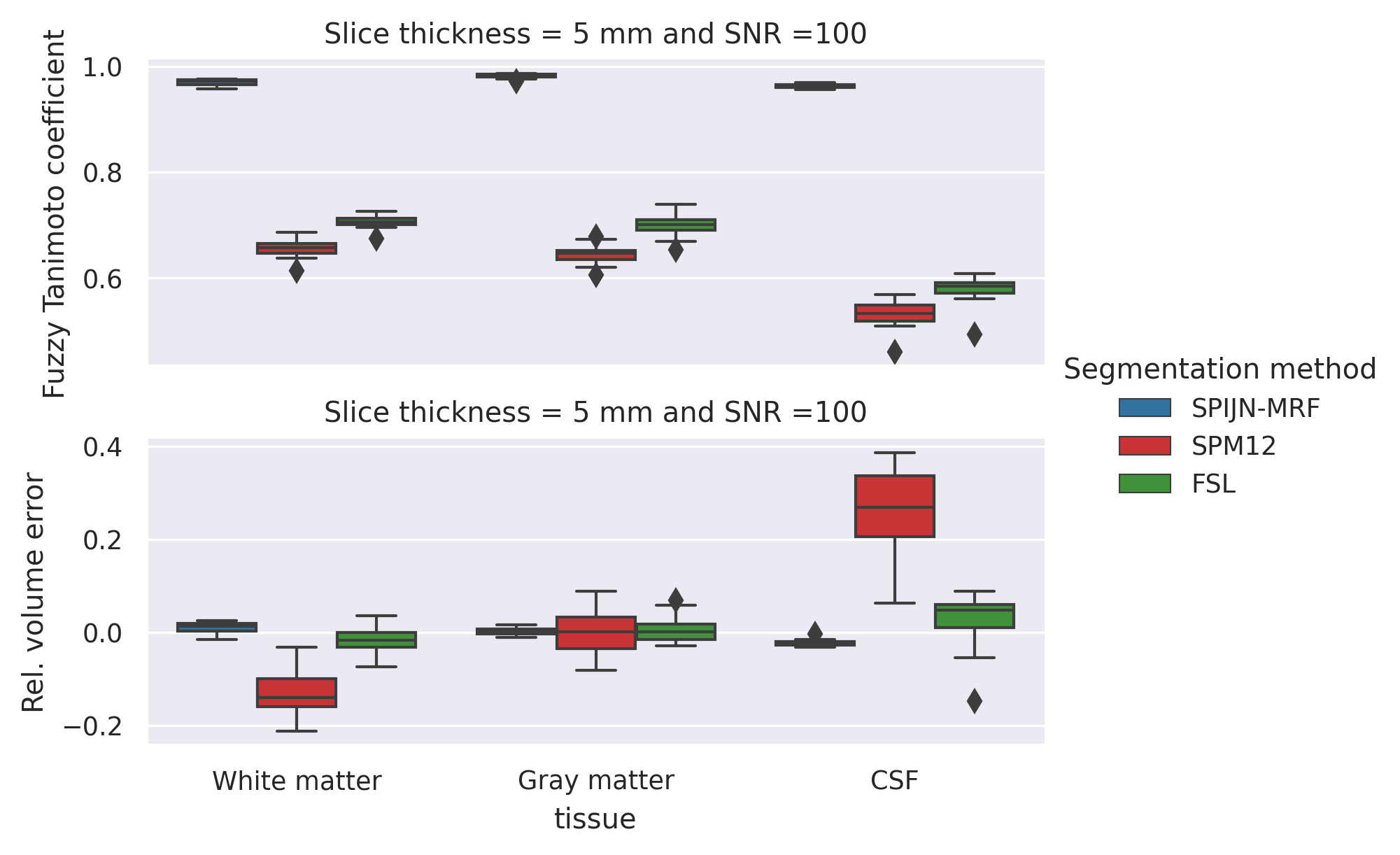
Numerical resultsSPIJN-MRF yielded exact outcomes estimating the number of tissue components and corresponding relaxation times. The obtained segmentations were very close to the ground truth(Fig.1), while FSL and SPM12 showed a larger voxel-wise error. The relative error in volume was especially larger for SPM12.
In vivo results
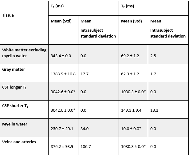
SPIJN-MRF T1 and T2-estimates showed to be highly repeatable for WM, GM and CSF(Table 1). In comparison, MW showed more variation in T1. Furthermore, T1-estimates for CSF consistently corresponded to the longest T1 in the dictionary.
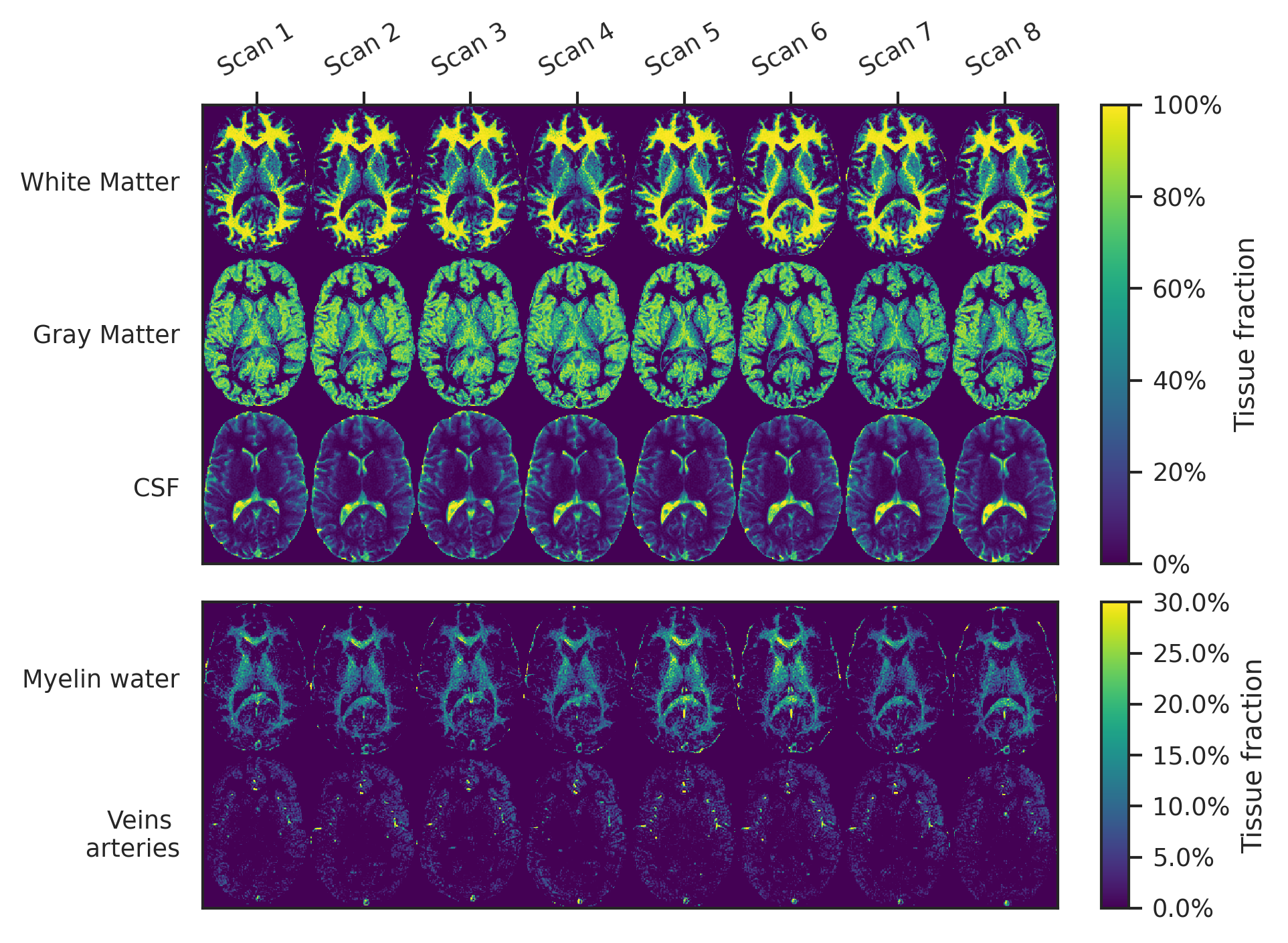
Magnetization fraction maps for one subject for a center slice are given in Fig.2, showing a high similarity between scans, although a slight variation in MW-fraction can be observed.
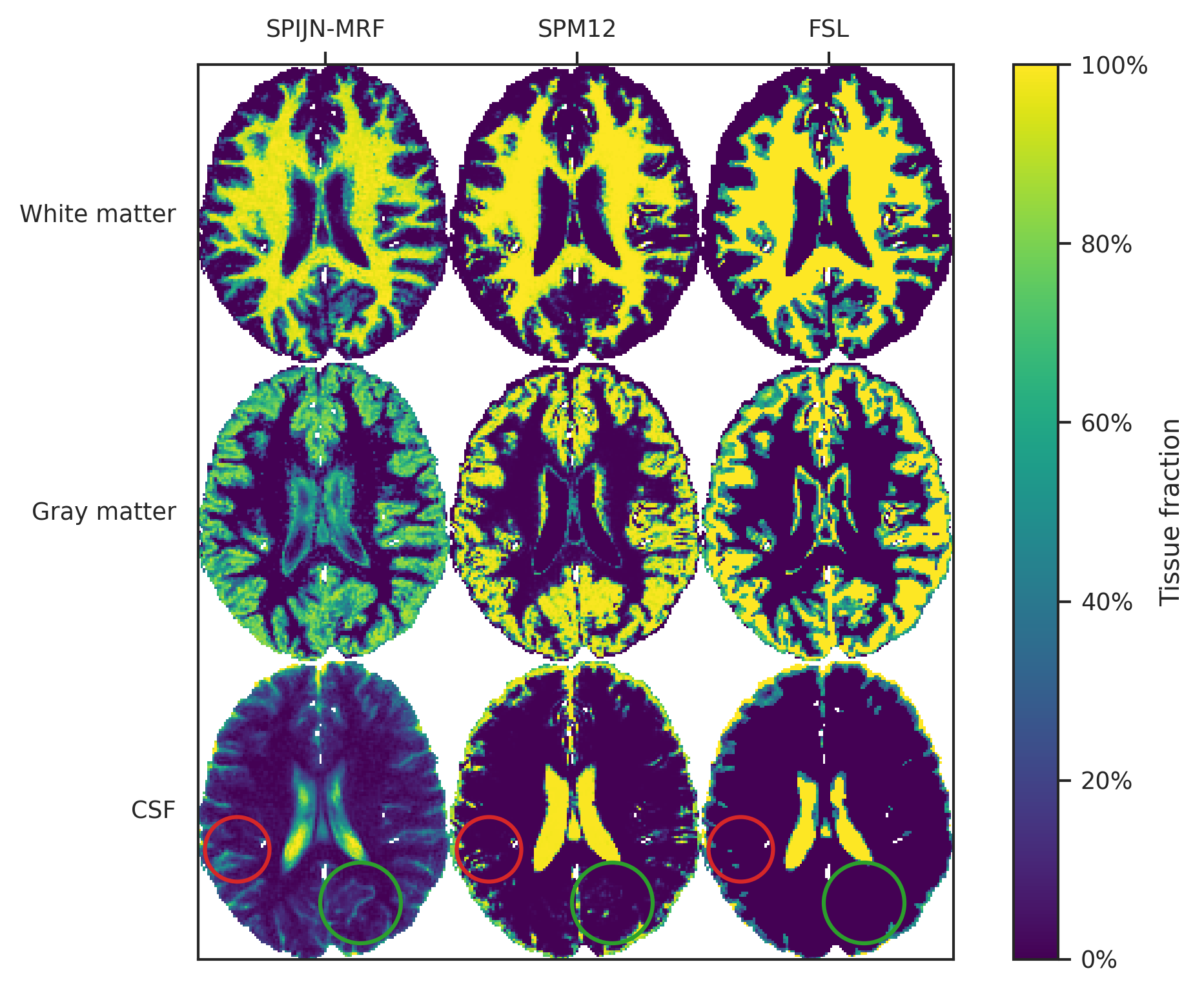
Segmentations obtained with SPIJN-MRF, SPM12 and FSL showed clear differences(Fig.3), especially in the CSF and partial volume regions.
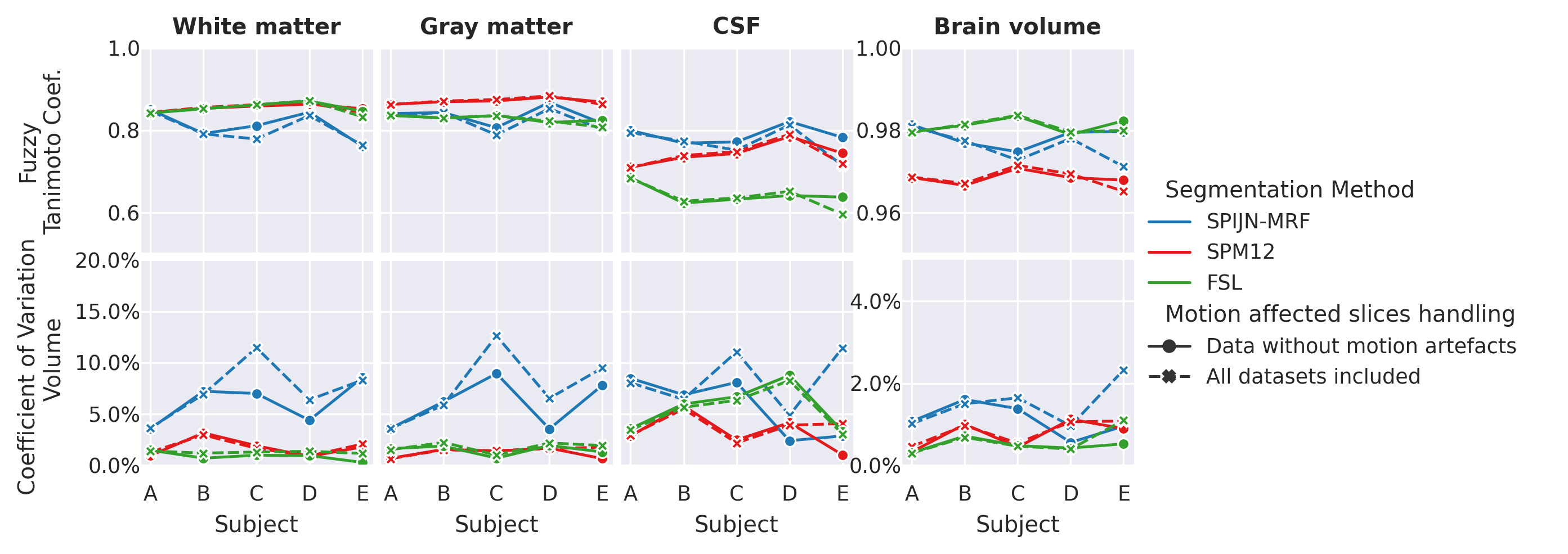
Fig.4 shows the estimated CFTC and CoV. SPM12 and FSL yielded smaller CoVs than SPIJN-MRF for WM and GM, while differences were smaller for CSF and Brain volume. Differences in CTFC were smaller and for CSF SPIJN-MRF showed better scores than SPM12 and FSL.
Discussion
The estimated relaxation times by SPIJN-MRF were in line with previously reported values12, but WM(excluding MW) showed higher T2 than GM, possibly due to the identification of as a separate component .In simulations, SPIJN-MRF showed a very small bias in total volume estimates and very high FTC compared with SPM12 and FSL. In vivo, SPM12 and FSL segmentations showed a very low CoV, also compared to previous studies13,14, this could be caused by the use of sT1w-images, potentially leading to artificially increased reproducibility (and possibly at the expense of biased estimates).
Conclusion
SPIJN-MRF is able to estimate accurate and precise tissue relaxation times and partial volume maps with increased accuracy in CSF compared to conventional methods.Acknowledgements
This research was partly funded by the Medical Delta consortium, a collaboration between the Delft University of Technology, Leiden University, Erasmus University Rotterdam, Leiden University Medical Center and Erasmus Medical Centre. This research was partially financed by a Research Grant from GE (B-GEHC-05).References
(1) Ma, D.; Gulani, V.; Seiberlich, N.; Liu, K.; Sunshine, J. L.; Duerk, J. L.; Griswold, M. A. Magnetic Resonance Fingerprinting. Nature 2013, 495 (7440), 187–192. https://doi.org/10.1038/nature11971.
(2) McGivney, D. F.; Boyacıoğlu, R.; Jiang, Y.; Poorman, M. E.; Seiberlich, N.; Gulani, V.; Keenan, K. E.; Griswold, M. A.; Ma, D. Magnetic Resonance Fingerprinting Review Part 2: Technique and Directions. Journal of Magnetic Resonance Imaging 2019, 0 (0). https://doi.org/10.1002/jmri.26877.
(3) Nagtegaal, M. A.; Koken, P.; Amthor, T.; Doneva, M. Fast Multi-Component Analysis Using a Joint Sparsity Constraint for MR Fingerprinting. Magnetic Resonance in Medicine 2020, 83 (2), 521–534. https://doi.org/10.1002/mrm.27947.
(4) McGivney, D.; Deshmane, A.; Jiang, Y.; Ma, D.; Badve, C.; Sloan, A.; Gulani, V.; Griswold, M. Bayesian Estimation of Multicomponent Relaxation Parameters in Magnetic Resonance Fingerprinting: Bayesian MRF. Magnetic Resonance in Medicine 2017. https://doi.org/10.1002/mrm.27017.
(5) Tang, S.; Fernandez-Granda, C.; Lannuzel, S.; Bernstein, B.; Lattanzi, R.; Cloos, M.; Knoll, F.; Assländer, J. Multicompartment Magnetic Resonance Fingerprinting. Inverse Problems 2018, 34 (9), 094005. https://doi.org/10.1088/1361-6420/aad1c3.
(6) Aubert-Broche, B.; Griffin, M.; Pike, G. B.; Evans, A. C.; Collins, D. L. Twenty New Digital Brain Phantoms for Creation of Validation Image Data Bases. IEEE Transactions on Medical Imaging 2006, 25 (11), 1410–1416. https://doi.org/10.1109/TMI.2006.883453.
(7) Jiang, Y.; Ma, D.; Seiberlich, N.; Gulani, V.; Griswold, M. A. MR Fingerprinting Using Fast Imaging with Steady State Precession (FISP) with Spiral Readout. Magnetic Resonance in Medicine 2015, 74 (6), 1621–1631. https://doi.org/10.1002/mrm.25559.
(8) Hennig, J. Multiecho Imaging Sequences with Low Refocusing Flip Angles. Journal of Magnetic Resonance 1988, 78 (3), 397–407. https://doi.org/10.1016/0022-2364(88)90128-X.
(9) Jenkinson, M.; Beckmann, C. F.; Behrens, T. E. J.; Woolrich, M. W.; Smith, S. M. FSL. NeuroImage 2012, 62 (2), 782–790. https://doi.org/10.1016/j.neuroimage.2011.09.015.
(10) Ashburner, J.; Friston, K. J. Unified Segmentation. NeuroImage 2005, 26 (3), 839–851. https://doi.org/10.1016/j.neuroimage.2005.02.018.
(11) Crum, W. R.; Camara, O.; Hill, D. L. G. Generalized Overlap Measures for Evaluation and Validation in Medical Image Analysis. IEEE Transactions on Medical Imaging 2006, 25 (11), 1451–1461. https://doi.org/10.1109/TMI.2006.880587.
(12) Bojorquez, J. Z.; Bricq, S.; Acquitter, C.; Brunotte, F.; Walker, P. M.; Lalande, A. What Are Normal Relaxation Times of Tissues at 3 T? Magnetic Resonance Imaging 2017, 35, 69–80. https://doi.org/10.1016/j.mri.2016.08.021.
(13) Klauschen, F.; Goldman, A.; Barra, V.; Meyer-Lindenberg, A.; Lundervold, A. Evaluation of Automated Brain MR Image Segmentation and Volumetry Methods. Human Brain Mapping 2009, 30 (4), 1310–1327. https://doi.org/10.1002/hbm.20599.
(14) Tudorascu, D. L.; Karim, H. T.; Maronge, J. M.; Alhilali, L.; Fakhran, S.; Aizenstein, H. J.; Muschelli, J.; Crainiceanu, C. M. Reproducibility and Bias in Healthy Brain Segmentation: Comparison of Two Popular Neuroimaging Platforms. Frontiers in Neuroscience 2016, 10, 503. https://doi.org/10.3389/fnins.2016.00503.
Figures