Introduction

Magnetic Resonance Fingerprinting¹ (MRF) is a novel method for simultaneous multi-parametric quantitative image acquisition. Since the discovery of MRF, developments have been made to increase the precision and accuracy of quantitative maps^2-4 and to decrease the time required for data acquisition and computation^4-6. In addition to dictionary matching, maximum likelihood² and interpolation³ algorithms have been used to further refine parameter retrieval. These algorithmic approaches no longer constrain MR parameters to the discrete values contained within the dictionary. By the same motivation, we implement a non-linear optimization algorithm, initialized by dictionary matching, and perform a Monte Carlo error analysis to inspect the influence of signal-to-noise ratio (SNR) on the performance of non-linear optimization. Additionally, we demonstrate the feasibility of using a sparse dictionary alongside non-linear optimization to provide results comparable to a dense dictionary with non-linear optimization.

Methods

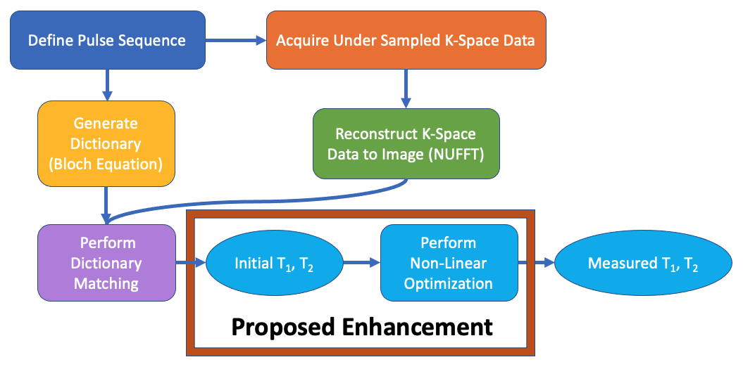
We modify the MRF pipeline (Figure 1) by inserting non-linear optimization as a step after dictionary matching. With this modification, we test the robustness of non-linear optimization with respect to noise in a Monte Carlo simulation and assess the opportunity to use smaller dictionary sizes. The MRF measurements in our study were computed by simulation.

Non-linear Optimization:
We minimize $$$T_1$$$ and $$$T_2$$$ in a least squares sense
$$\min_{T_1, T_2} || \mathbf{v} - \rho \mathbf{b}(T_1, T_2)||^2$$
Where $$$\mathbf{v}$$$ is the measured signal, $$$\mathbf{b}$$$ is the modeled signal as determined by the Bloch equation, and $$$\rho$$$ is the proton density. For a given $$$T_1$$$ and $$$T_2$$$, there exists an optimal value for $$$\rho$$$ given by a linear analytical solution.
$$\rho_{opt} = \frac{1}{||\mathbf{b}||^2} \left(\mathbf{b_r}\cdot\mathbf{v_r} + \mathbf{b_i}\cdot\mathbf{v_i} + i\left(\mathbf{b_r}\cdot\mathbf{v_i} - \mathbf{b_i}\cdot\mathbf{v_r}\right)\right).$$
We use the above equations along with the MATLAB built-in function, fminsearch, to evaluate the first equation.

Monte Carlo:
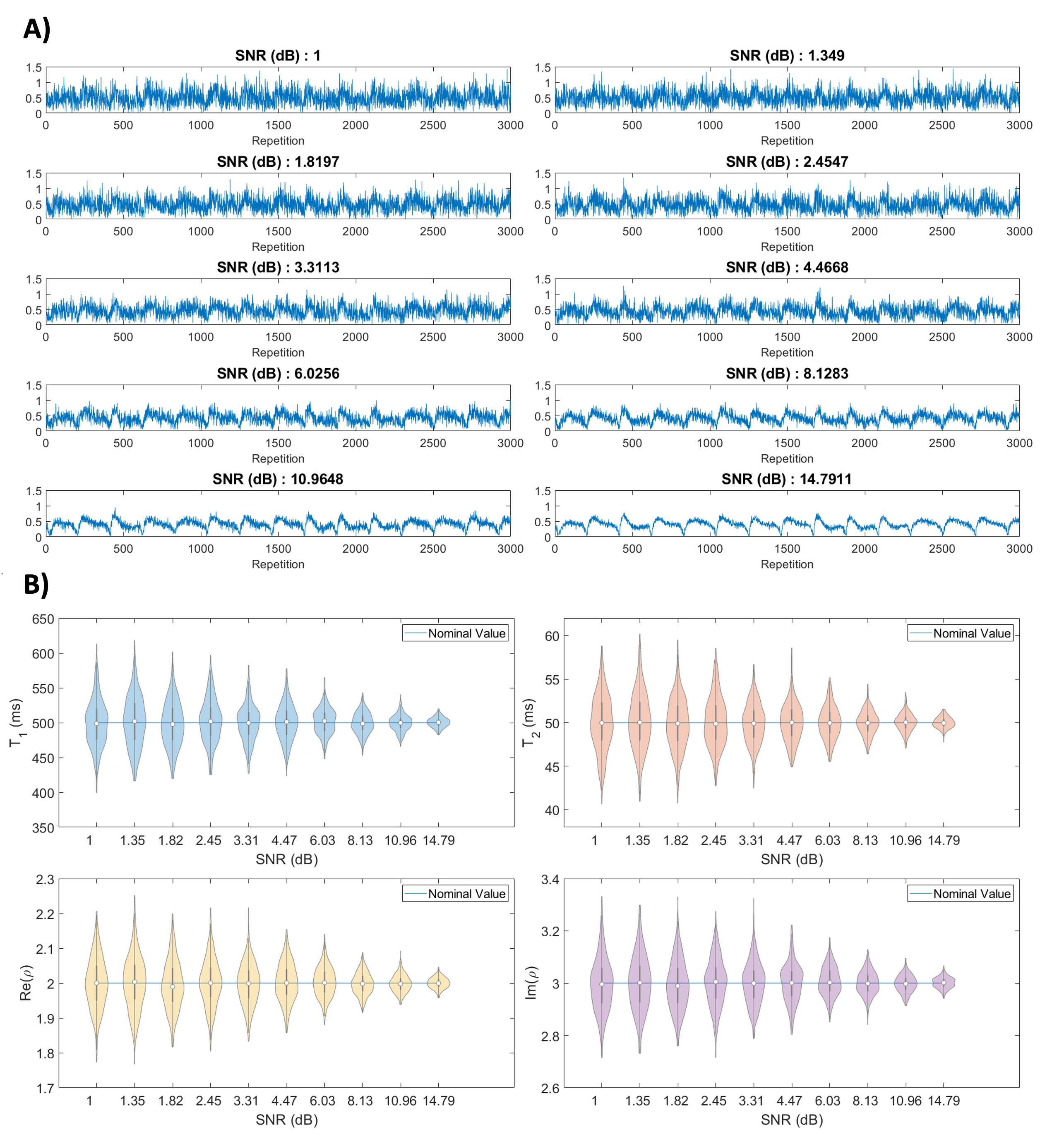
In the Monte Carlo simulation, we imitate a measured signal by inserting Gaussian noise into a signal generated from a Bloch solver; the width of the Gaussian noise is determined by the SNR level, $$$ SNR = 10\log_{10}\left(\frac{||\mathbf{v}||^2}{n\sigma^2}\right)$$$, where $$$\mathbf{v}$$$ is the measured signal, $$$n$$$ is the number of time points, and $$$\sigma$$$ is the width of the Gaussian noise. We choose arbitrary nominal values for $$$T_1$$$, $$$T_2$$$, and proton density of 500ms, 50ms, and $$$2 + 3i$$$ respectively. In the experiment, we select 10 levels of SNR and perform 720 Monte Carlo realizations at each level. In a single realization, we generate and insert complex Gaussian noise into the nominal signal, initialize $$$T_1$$$ and $$$T_2$$$ to $$$\pm 10$$$ms from their nominal value, perform non-linear optimization, and record the parameter values after optimization.

MRF Simulation:
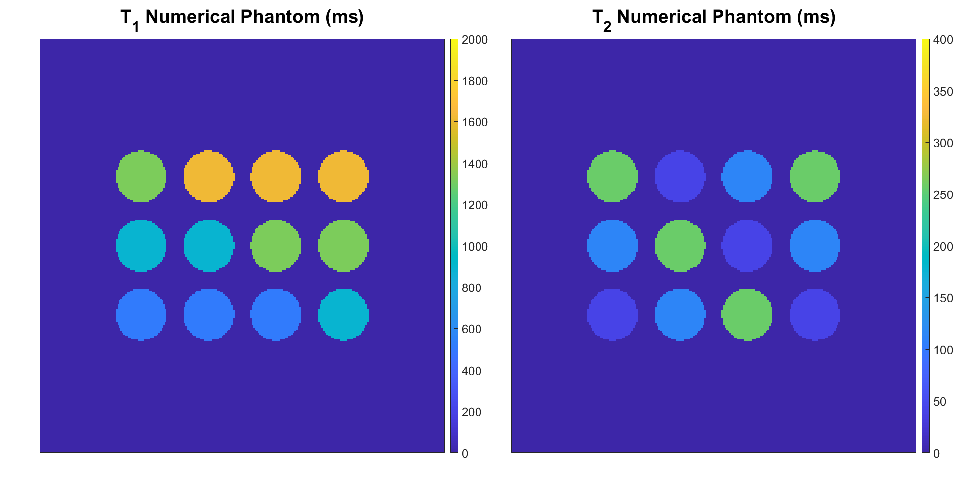
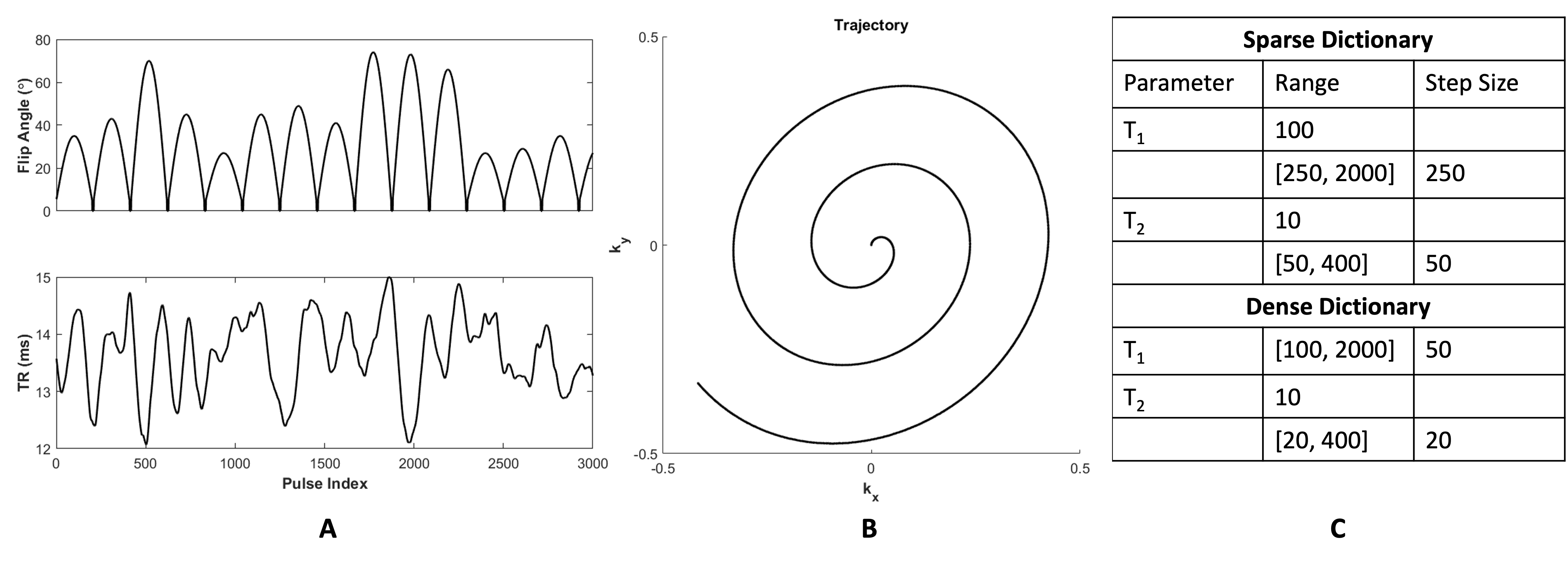
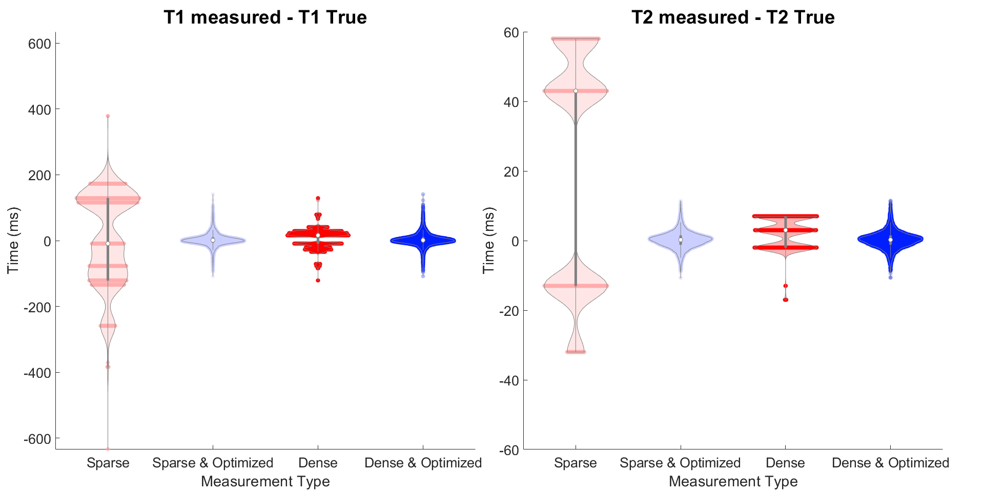
To assess the opportunity to use smaller dictionary sizes, we simulate MRF using a numerical phantom (Figure 2). We use an SSFP sequence with undersampled spiral readout (Figure 3A-B). We run the MRF simulation using dictionary matching alone and using dictionary matching with optimization; for each of these, we use both densely populated and sparse dictionaries (Figure 3C). We plot the distributions of the residuals and compare results.

Results and Discussion

Figure 4A shows the varying levels of noise used in the Monte Carlo experiment, and Figure 4B shows the resulting distributions after 720 minimizations at each noise level. First, we observe unbiased distributions centered around the nominal value for each parameter. We also observe the variance decreasing as the signal increases. These results suggest non-linear optimization is robust with respect to noise.

Figure 5 shows the distribution of the residuals resulting from four methods of simulating MRF on the numerical phantom. From the distributions that include optimization, we notice they are centered around zero and are normally distributed. This suggests optimization is well-behaved and produces accurate results. We also notice that when using optimization, the distributions are almost identical, independent of the dictionary type used. This suggests non-linear optimization converges to a global minimum over a wide range of initial conditions and is robust with respect to initial conditions. In turn, with optimization, smaller dictionary sizes could be used, reducing the computer memory and computation time required for dictionary matching. The time savings in dictionary matching would then be used in non-linear optimization where more accurate parameter measurements may be made, as we are no longer confined to the discrete grid of dictionary entries. Further research will include enhancements to the non-linear optimization algorithm to increase the computational efficiency.

Conclusion

These findings provide a basis for improving the accuracy and efficiency of the MRF pipeline and give insight into quantifying error propagating through the pipeline. The results suggest that non-linear optimization performs well in the presence of noise; that non-linear optimization can be used in combination with smaller dictionary sizes; and that non-linear optimization has the potential to reduce memory requirements while producing more accurate results.

Acknowledgements

This work was performed under financial assistance award 70NANB18H006 from the U.S. Department of Commerce, National Institute of Standards and Technology and from the Summer Undergraduate Research Fellowship.