1 Introduction

We present an efficient spiral MR Fingerprinting¹ protocol for quantitative imaging of the prostate at 3T in less than five minutes. Compared to previously presented prostate MRF protocols^2,3 we use an additional chemical shift based water/fat separation (Dixon-MRF), and perform a fully-integrated DREAM pre-scan for B₁⁺ correction in MRF. The fast reconstruction using the scanner’s built-in GPU allow MRF parameter maps to be reconstructed on the console without disturbing the clinical workflow.

2 Methods

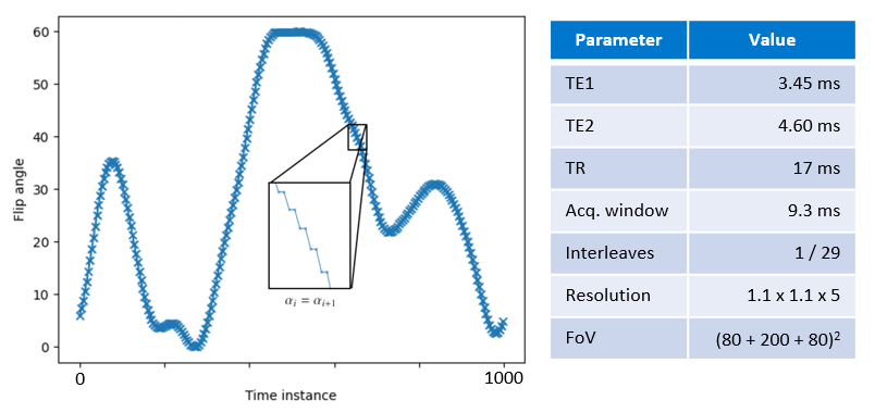
2.1 MRF acquisition & reconstruction
An MRF protocol of 15 slices (slice thickness 5 mm), FoV of 200 x 200 mm² with 80 mm oversampling (in-plane resolution of 1.1 mm) has been designed for full coverage of the prostate. A flip angle train of length 1000 with interleaved echo times⁴ and TR = 17 ms is used, cf. Figure 1. For each flip angle, a single-spiral with undersampling of 29 was aquired. Joint spiral deblurring and water/fat separation⁵ is performed on each data tuple along the MRF train. The resulting water-only (fat-suppressed) MRF images are matched against a dictionary with T₁ = [0, 3000] ms, T₂ = [0, 1000] ms (both discretized on a log-scale of 2% step size), and B₁⁺ = [0.75, 1.25] with at linear step size of 1%. The MRF reconstruction was integrated in the scanner software using a GPU backend that resulted in a latency of less than ten seconds for the multi-slice acquisition.
Additionally, we apply flow compensation where an extra gradient in slice selection direction is added such that its first moment vanishes and, thus, flow of constant through-plane velocity is expected to cancel out.

2.2 Protocol details
Our protocol consists of the following fully-integrated steps:

(i) A volumetric DREAM⁶ pre-scan (similar to a B₀ pre-scan performed for, e.g., spiral deblurring) for B₁⁺ measurement on a coarser and larger geometry compared to (ii) is acquired in a multi 2D acquisition (FoV = 470 x 470 mm², slices = 20, slice thickness = 10 mm, pixel size = 5.88 mm, TR = 4.1 ms, averages = 4, Uniformity = ’CLEAR’, STEAM angle = 80, total scan time = 01:07 min). An RF Shim volume is placed in the area of the prostate in order to achieve a homogeneous map ∼ 100% in that body region.

(ii) Multi 2D MR-Fingerprinting as described in Subsection 2.1 with joint spiral deblurring and water/fat separation according to Wang⁵. The map obtained in (i) is automatically interpolated onto the present geometry, and is used for corrected dictionary matching.

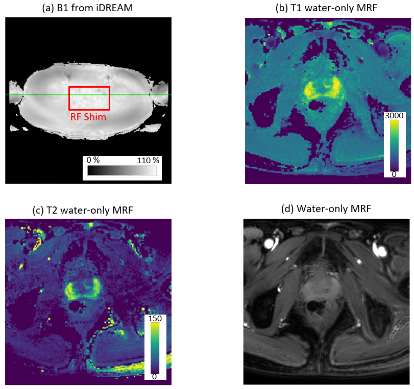
The suggested prostate MRF protocol consists of the scans (i) and (ii), and a typical output for the fat-suppressed case is shown in Figure 2. T₁ and T₂ maps of the prostate of six healthy volunteers (informed consent obtained) have been obtained on a 3T MRI system (Ingenia, Philips Healthcare). Additionally, a 2D multi-echo spin-echo scan for T₂ comparison was performed:

(iii) 2D multi-echo spin-echo (MESE) scan located at a relevant slice obtained in (ii) for T₂ reference. Parameters: TR = 5 s, 14 echoes, TEn = n*16 ms, 160$$$^\circ$$$ constant refocusing, acquisition voxel 0.96 x 0.96 x 3 mm³, oversampling 135 mm, Compressed SENSE R=7, total single slice scan time = 06:00 min.

3 Results and Discussion

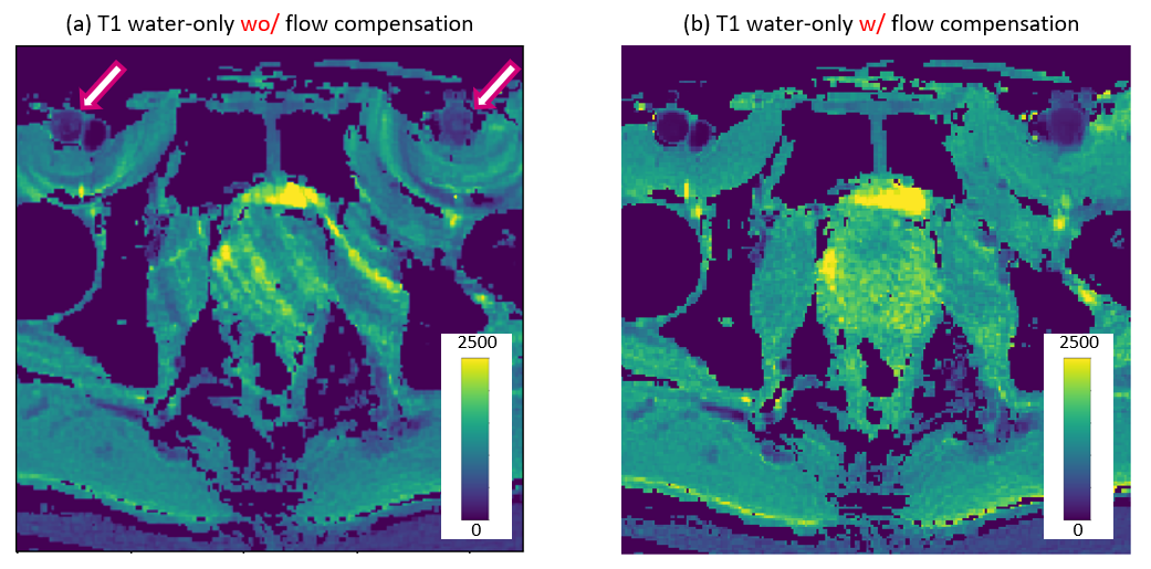
The presented prostate Dixon-MRF protocol has been optimized with respect to overall scan time and resolution. In Figure 3, we show a comparison between MRF with and without flow compensation for a single volunteer. We note strong spiral artifacts that cause rings centered around both arteries affecting the T₁ values in the prostate. Flow compensation leads to a much smaller and more local effect of the blood flow and, thus, corrects the values of T₁/T₂ in the prostate. B₁⁺ correction was performed in all cases. The placement of the RF Shim volume yields values near 100% in the prostate with larger variations in other body parts, cf. Figure 2(a).
Figure 4 shows T₁, T₂ MRF and the reference MESE T₂ map for all considered volunteers. A good agreement of the respective T₂ distribution is observed. The discrepancy in T₂ magnitudes comparing water/fat resolved MRF and the MESE reference in Figure 4 may be explained by a combination of stimulated echo effects (prolonging T₂ results in MESE⁷) and magnetization transfer effects, prolonging T₂-MESE and shortening T₂ results in MRF, because they are not considered for the dictionary (this would require a 2-pool model⁸).
Figure 5 shows the MRF T₂ values evaluated in the normal-appearing peripheral zone (NPZ) for all six volunteers. We note a strong variation in T₂ in the considered ROI over all volunteers but observe a nearly linear behaviour when comparing to the MESE values.

4 Conclusion

A high-quality, high SNR, prostate MRF protocol with additional B₁⁺ correction from a fully-integrated DREAM scan (+1 min) in less than 5 mins is presented. The extension by a robust water/fat separation can be used especially in regions where fat-induced blurring affects the image quality. We further provided an instantaneous reconstruction workflow that makes the new protocol attractive in clinical practice. A comparison with (standard) MESE T₂ mapping (single-slice acquisition in 6 mins) shows good correlation with the maps obtained from MRF and give confidence for evaluation in further clinical studies.

Acknowledgements

We would like to thank Victoria Yu, Can Wu, Ouri Cohen, Ergys Subashi, and Ricardo Otazo from MSKCC for helpful discussions on the topic.