2559
Comparison of 2D vs 3D Deep Learning Algorithms to Estimate Temperature Throughout the Human Body
Giuseppe Carluccio1, Eros Montin1, Riccardo Lattanzi1, and Christopher Michael Collins1
1Center for Advanced Imaging Innovation and Research (CAI2R), New York, NY, United States
1Center for Advanced Imaging Innovation and Research (CAI2R), New York, NY, United States
Synopsis
We developed and compared two different Deep-Learning (DL) based approaches to approximating temperature in subject-specific body models. The first involved use of a 2D U-net to predict temperature throughout the body on a slice-by-slice basis, and the second involved use of a 3D U-net to predict temperature in the 3D body. The 3D approach greatly outperformed the 2D approach, and was very fast.
Introduction
In MRI, radiofrequency (RF) fields used to excite the nuclei and generate a detectable signal also produce RF electric fields which generate heat in conductive tissues. Therefore, safety limits have been imposed on the maximum local or whole-body Specific energy Absorption Rate (SAR), and on the core and local temperature1. RF safety assurance in MRI relies heavily on numerical simulations to estimate SAR and temperature, where a human body model is simulated with the RF coil used in imaging.Because of the limited availability of numerical human models and difficulty in producing patient-specific models and associated field simulations in a reasonable time2, there has been some interest in the potential for Deep Learning (DL) algorithms to predict patient-specific SAR for MRI3,4. For example, Meliado et al.3 have presented a method where a neural network can estimate the SAR distribution from a transmit array with B1+ maps used as an input. Recently, Gokyar et al.4 have developed a neural network able to estimate the SAR distribution starting from approximated MR images (model water content weighted by the transmit B1+ field). In both publications 2D neural networks were used to predict SAR. However, temperature is more directly related to risk. To our knowledge, no publication has been presented to estimate temperature within the human body using deep learning algorithms. In this work, we evaluate the efficacy of neural networks when estimating the baseline temperature throughout the patient starting from body tissue property maps in lieu of rapidly-acquired images. Specifically, we compare the accuracy when 2D vs. 3D deep learning networks are used to predict temperature throughout the model.Methods
DataWe designed two neural networks able to estimate the baseline temperature starting from atlas maps. The ground truth temperature is calculated with a in-house C++ simulator of the bioheat equation $$\rho c \frac{\partial T}{\partial t}=\nabla (k \cdot \nabla T)- \rho_{bl} c_{bl} W (T-T_{bl})+Q+SAR $$ where $$$T$$$ is the temperature, $$$c$$$ is the heat capacity, $$$W$$$ is the blood perfusion rate, $$$k$$$ is the thermal conductivity, $$$\rho$$$ is tissue mass density, $$$Q$$$ is the heat generated by metabolism. The subscript $$$bl$$$ indicates values for blood. The atlas maps were derived from 6 body models: Duke and Ella of the Virtual Family5, Naomi6 and Norman7, and models produced from the NLM Male and the NLM Female Visible Human Project datasets8,9. To train and test the 2D algorithms, data from many different slices of the models were used. To train and test the 3D algorithms, additional body models were created by scaling the models by different factors in different directions to produce a total of 1296 different body models. Inputs and outputs for the two approaches are described in Figure 1: a series of JPG images for the 2D network (three channels), and a 4D tensor (5 channels with a 3D matrix on each) for the 3D network.
Networks
We have designed two neural networks, one using 2D filters, and one using 3D filters. Details of the employed U-nets are provided in Figure 1 and Figure 2. The body models Duke, Ella, NLM Male, and NLM Female were used for training, while the remaining two models, Naomi and Norman, were used for the testing validation. The training of both networks was performed with a leave-one-out cross-validation approach with a learning rate of 0.1 for the 2D network, and 0.02 for the 3D network, mean squared error loss, and 10 training epochs. The performance of the two networks was evaluated by computing the percent Mean Square Error (MSE) between the computed baseline temperature through simulations and the estimated temperature with the neural networks on the test data.
Results and Discussion
There was a significant difference in performance between the two networks. Although the 2D network could provide results that appear qualitatively reasonable, it yielded a minimum percent MSE of 260%, and a maximum one of 1200% over the 3D volume. Also, when 2D results are assembled to create a 3D structure, there are discontinuities in sagittal and coronal views. The 3D network provided results very similar to the target baseline temperature so that the minimum and maximum percent MSE were equal to 0.02% and 0.2%, respectively. In addition, it provided consistent results in axial, coronal, and sagittal views. This should not be too surprising, considering that heat flows in all 3 directions, and therefore characterizing the heat distribution with 3D matrices can provide a superior estimation of the baseline temperature. In our implementation, the trained network can estimate a full 3D temperature distribution in less than 2 seconds for the entire body volume.Conclusions
A 3D deep learning neural network can be used to dramatically accelerate temperature estimation for the purpose of real-time patient-specific safety assessment with much greater accuracy than a 2D-based network. In the near future, we will apply these networks to estimate the temperature increase above baseline due to SAR absorption and utilize more MRI-specific input data.Acknowledgements
This work was performed under the rubric of the Center for Advanced Imaging Innovation and Research (CAI2R, www.cai2r.net) at the New York University School of Medicine, which is an NIBIB Biomedical Technology Resource Center (NIH P41 EB017183) with additional funding from NIH R01 EB021277 and NIH R01 EB024536.References
- International Electrotechnical Commission. “International standard, medical equipment – part 2: particular requirements for the safety of magnetic resonance equipment for medical diagnosis,” 3rd revision. (2010).
- Homann H et al. “Toward individualized SAR models and in vivo validation. Magnetic resonance in medicine.” 2011 Dec;66(6):1767-76.
- Meliadò EF et al. “A deep learning method for image‐based subject‐specific local SAR assessment. Magnetic resonance in medicine.” 2020 Feb;83(2):695-711.
- Gokyar S et al. MRSaiFE: An AI-Based Approach Towards the Real-Time Prediction of Specific Absorption Rate. IEEE Access. 2021 Oct 5;9:140824-34.
- Christ A et al. “The Virtual Family—development of surface-based anatomical models of two adults and two children for dosimetric simulations.” Physics in Medicine & Biology. 2009 Dec;55(2):N23
- Dimbylow PJ. “FDTD calculations of the whole-body averaged SAR in an anatomically realistic voxel model of the human body from 1 MHz to 1 GHz.” Physics in Medicine & Biology. 1997 Mar;42(3):479.
- Dimbylow P. “Development of the female voxel phantom, NAOMI, and its application to calculations of induced current densities and electric fields from applied low frequency magnetic and electric fields.” Physics in Medicine & Biology. 2005 Feb 23;50(6):1047.
- Collins CM, Smith MB. “Calculations of B1 distribution, SNR, and SAR for a surface coil adjacent to an anatomically‐accurate human body model.” Magnetic Resonance in Medicine: An Official Journal of the International Society for Magnetic Resonance in Medicine. 2001 Apr;45(4):692-9.
- Liu W, Collins CM, Smith MB. “Calculations of B1 distribution, specific energy absorption rate, and intrinsic signal-to-noise ratio for a body-size birdcage coil loaded with different human subjects at 64 and 128 MHz.” Applied magnetic resonance. 2005 Mar 1;29(1):5.
Figures
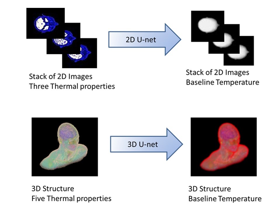
Figure 1: Description of the designed inputs/outputs. The 2D U-net was trained using as input a 2D data loader based on JPG images where c was assigned to the red channel, W to the green channel. and Q to the blue channel. The output images contain the baseline temperature distribution as a series of grayscale JPG images. The 3D network uses 3D structures: it has 5 input channels corresponding to the thermal properties of c, W, k, ρ, and Q, and one output corresponding to the baseline temperature.
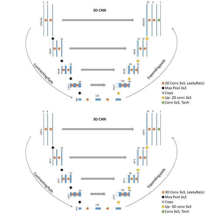
Figure 2. The architecture of the used neural networks. Blue rectangles represent feature maps with the size and the number of feature maps indicated on top of the bins. Different operations in the network are depicted by color-coded arrows. Eight feature maps were used in the first and last layer of the network, 4 path layers, and leakyRelu as activation functions. The input size of the 2D-Unet was 140x140 while 3D-Unet 128x128x128 and zero-padding were used for convolutions.
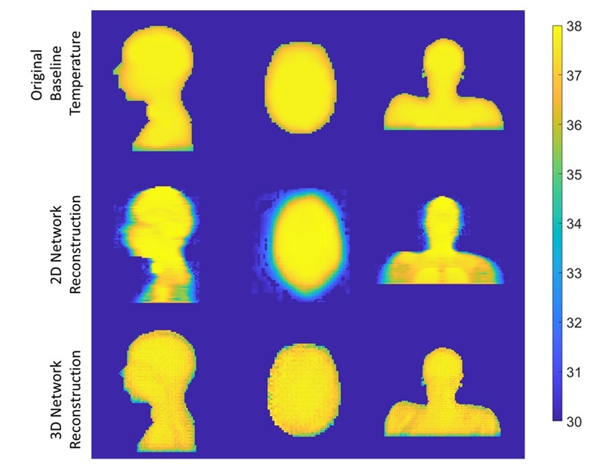
Figure 3: Comparisons of the performance between the two developed networks, with respect to the simulated baseline temperature (top row), for 3 different orthogonal views. The images inferred with the 2D U-net (middle row) have a percent MSE of 271% , while the structure inferred with the 3D U-net (bottom row) has a percent MSE of 0.06%.
DOI: https://doi.org/10.58530/2022/2559