2541
Denoising MR spectra by deep learning: miracle or mirage?
Martyna Dziadosz1,2, Rudy Rizzo1,2, Sreenath P Kyathanahally3, and Roland Kreis1,2
1Magnetic Resonance Methodology, Institute of Diagnostic and Interventional Neuroradiology, University of Bern, Bern, Switzerland, 2Translational Imaging Center, sitem-insel, Bern, Switzerland, 3Department Systems Analysis, Integrated Assessment and Modelling, Data Science for Environmental Research group, Dübendorf, Switzerland
1Magnetic Resonance Methodology, Institute of Diagnostic and Interventional Neuroradiology, University of Bern, Bern, Switzerland, 2Translational Imaging Center, sitem-insel, Bern, Switzerland, 3Department Systems Analysis, Integrated Assessment and Modelling, Data Science for Environmental Research group, Dübendorf, Switzerland
Synopsis
The main limitation of MRS is low SNR. Several approaches for denoising have been proposed. However, it is debatable, whether denoising can reduce estimate uncertainties. In this work, we investigate denoising using deep learning (DL) in time-frequency representations. The results were assessed using two methods: first, an adjusted noise score was used and second, the outcome of traditional fitting was evaluated. We found that time-frequency domain denoising through DL produces a visually appealing spectrum but mean residuals for the relevant spectral regions and variance in fit results remained as high as without denoising.
Introduction
Magnetic Resonance Spectroscopy (MRS) is mainly limited by poor signal to noise (SNR)1-3. This is aggravated for low-concentration metabolites, such as GABA or scyllo-inositol. Therefore, to improve SNR several denoising techniques have been proposed: apodization4, signal decomposition5,6, wavelet feature analysis7,8 or principal component analysis9,10.However, it is still disputed whether denoising can reduce estimation uncertainties or whether it is only a cosmetic tool lowering noise in signal-free areas. In settings with multiple spectra, denoising methods based on spatial-spectral (or dynamic-spectral) separability have been shown to have the potential to reduce uncertainty for fitted metabolite content11. However, for single spectra it is unclear whether deep learning (DL) based methods that have shown benefits in image denoising or for distortion corrections could reduce uncertainties in spectral fitting. In particular, we explore denoising by DL in a time-frequency representation of spectroscopy data, where signal as well as noise is spread out into two dimensions, where a neural network might disentangle noise from signal more efficiently than in either single domain. We evaluate effectiveness of denoising using two approaches, first just using an adapted noise score and second by judging the outcome of traditional (‘gold-standard’) fitting.
Methods
Spectra mimicking human brain spectra were generated in VESPA12 (TE=35ms sLASER13). The datasets contain 16 metabolites with concentrations varying from 0 to double that seen in healthy brain14. A constant water reference is added at 0.5 ppm to ease quantification. To imitate in vivo conditions, the following parameters were varied: shim 2-5Hz, water SNR 5-40, and macro-molecular background14 by ±33%.A short-time Fourier transform with window size 128 and overlap interval of 97 was used to transform time-domain signals (4096 points, 1 s) into spectrograms, creating a 128x128 matrix.
The DL model - a U-net with symmetric skip connections (derived from 2D audio signal processing15) is detailed in Figure 1. It employs real and imaginary channels and projects original spectrograms into seemingly noise-free representations.
$$DQ = \frac{Σ_i(IGT_i - IDN_i)^2}{Σ_i(N_i)^2};\
DQ_w = \frac{Σ_i IGT_i^2(IGT_i - IDN_i)^2}{Σ_i(N_i)^2 IGT_i^2} \ $$
The denoising effect is quantified using a score called DQ (Denoising Quality), which is calculated as a weighted (DQw) or non-weighted (DQ) mean absolute deviation from ground truth (GT) compared to the mean absolute deviation from 0 for pure noise. DQ is equivalent to the fit quality score. Weighting with the GT spectrum renders this measure (DQw) sensitive to the relevant spectral regions.
Results & Discussion
According to visual evaluation, the novel MRS denoising approach implemented in the time-frequency domain performs extremely well as evident from Figure 2. However, to fully assess the actual efficacy of denoising DQ and DQw are presented in Figure 3 for a testset of 1k spectra. DQ evaluated for the whole spectral range is close to zero across a wide range of SNR and fairly small when restricted to the frequency range of interest, but DQw is close to one on average implying that denoising is mostly successful in non-signal comprising regions only.To better understand the effect of denoising, original (noisy) and denoised spectra were quantified using FitAID and results presented in Figure 4, which depicts the fitting estimates from noisy and denoised inputs for 16 metabolites as plotted against the GT concentration plus projection histograms next to the axes. Datapoints are color-coded by metabolite SNR (defined as the product of the spectral SNR (from water) and GT metabolite concentration) which can also be used to roughly summarize the denoising effect for three groups of metabolites:
(1) low metabolite SNR, where denoising seems successful because it prevents outliers and may thus lead to lower or similar mean fit deviations (sigma) but has a clear detrimental effect strongly biasing the fit results to a Gaussian distribution around the center of the training concentration range (e.g. Lac, Scy);
(2) medium metabolite SNR, where the prediction is less obviously but still biased by the training range (e.g. NAAG);
(3) high metabolite SNR, where fitting of the denoised and original spectra performs similarly with similar but never lower fitting bias (sigma) and where differences are less obvious (mI).
A more detailed evaluation is illustrated in Figure 5 for three exemplary metabolites.
Conclusions
We demonstrated that time-frequency domain denoising via DL is suitable for creating visually appealing spectra. However, the mean residuals for the relevant spectral areas appeared to be as high as when denoising is not employed. Based on the detailed evaluation including model fitting of denoised and noisy spectra and the variance of such results overall there is no gain from the developed DL-based denoising scheme. Care has to be taken in choosing the metric by which success of denoising is judged not to be misguided by the denoising effect in signal-free spectral areas and also not to be miraged by small fit errors for very low metabolite SNR data since DL denoising can introduce effective soft constraints for the allowed metabolite signal strength leading to fit results restricted to the training range of metabolite concentration from the denoising scheme.Acknowledgements
This work is supported by the Swiss National Science Foundation (SNSF #320030‐175984).References
- Zhang Y, Shen J. Effects of noise and linewidth on in vivo analysis of glutamate at 3 T. J Magn Reson. 2020; 314:106732.
- Macri MA, Garreffa G, Giove F, et al. In vivo quantitative 1H MRS of cerebellum and evaluation of quantitation reproducibility by simulation of different levels of noise and spectral resolution. Magn Reson Imaging. 2004; 22:1385-1393.
- Bartha R. Effect of signal-to-noise ratio and spectral linewidth on metabolite quantification at 4 T. NMR Biomed. 2007; 20:512-521.
- Goryawala M, Sullivan M, Maudsley AA. Effects of apodization smoothing and denoising on spectral fitting. Magn Reson Imaging. 2020; 70:108-114.
- Nguyen HM, Peng X, Do MN, Liang ZP. Denoising MR spectroscopic imaging data with low-rank approximations. IEEE Trans Biomed Eng. 2013; 60:78-89
- Liu Y, Ma C, Clifford BA, et al. Improved low-rank filtering of magnetic resonance spectroscopic imaging data corrupted by noise and B₀ field inhomogeneity. IEEE Transactions on Bio-medical Engineering. 2016; 63(4):841-849.
- Cancio-De-Greiff, Ramos-Garcia R, Lorenzo-Ginori JV. Signal De-noising in magnetic resonance spectroscopy using wavelet transforms. Concept Magnetic Res 2002; 14(6):388-401
- Ahmed OA. New denoising scheme for magnetic resonance spectroscopy signals. IEEE Trans Med Imaging. 2005; 24(6):809-16.
- Froeling M, Prompers JJ, Klomp DWJ, van der Velden TA. PCA denoising and Wiener deconvolution of 31P 3D CSI data to enhance effective SNR and improve point spread function. Magn Reson Med. 2021; 85:2992–3009.
- Jelescu IO, Veraart J, Cudalbu C. MP-PCA denoising dramatically improves SNR in large-sized MRS data: an illustration in diffusion-weighted MRS. In: Proc. Intl. Soc. Mag. Reson. Med. 28. 2020. p. 0395.Clarke WT, Chiew M. Uncertainty in denoising of MRSI using low- rank methods. Magn Reson Med. 2021 epub (DOI: 10.1002/mrm.29018).
- Oz G, Tkac I. Short-echo, single-shot, full-intensity proton magnetic resonance spectroscopy for neurochemical profiling at 4 T: validation in the cerebellum and brainstem. Magn Reson Med 2011; 65:901–910
- Marjanska, M., McCarten J.R., et al. Region-specific aging of the human brain as evidenced by neurochemical profiles measured noninvasively in the posterior cingulate cortex and occipital lobe using 1H magnetic resonance spectroscopy at 7T. Neuroscience 2017; 354:168-177
- Hoefemann, M., Adalid, V., Kreis, R. Optimizing acquisition and fitting conditions for 1H MR spectroscopy investigations in global brain pathology. NMR Biomed 2019; 32:e4161
- https://github.com/vbelz/Speech-enhancement
- Near J, Harris AD, Juchem C, et al. Preprocessing, analysis and quantification in single-voxel magnetic resonance spectroscopy: experts' consensus recommendations. NMR in Biomedicine. 2020; 32:e4257.
Figures
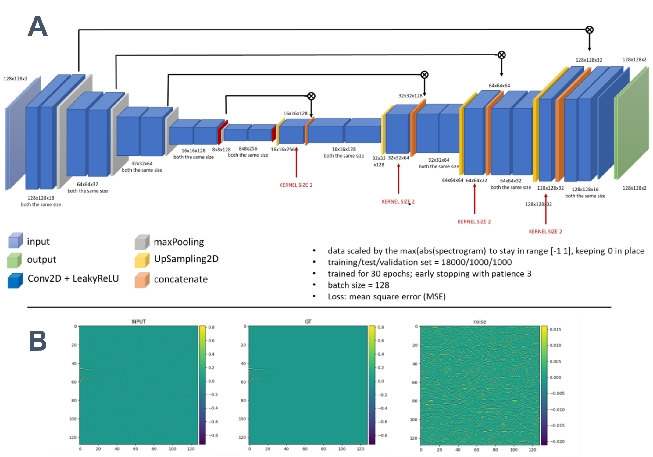
Figure 1. (A) The design of the U-net network with
details listed (parameters).
(B) Illustration of utilized datasets: 2D time-frequency
representation (spectrograms; 128x128 matrix) composed of two channels –
absorption and dispersion. From the left – noisy INPUT, noiseless GT and the
noise (INPUT-GT).
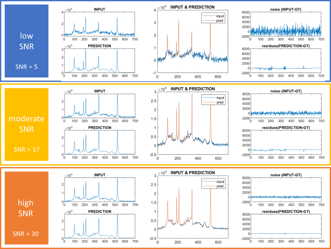
Figure 2. Illustrative
simulated spectra (INPUT) with low (upper row), moderate (middle row) and high
(lower row) SNR plotted with respective U-net reconstructed (denoised) spectra
(PREDICTION). Zoomed spectra are presented in the middle column. The right
column presents the noise before and after denoising (residues).
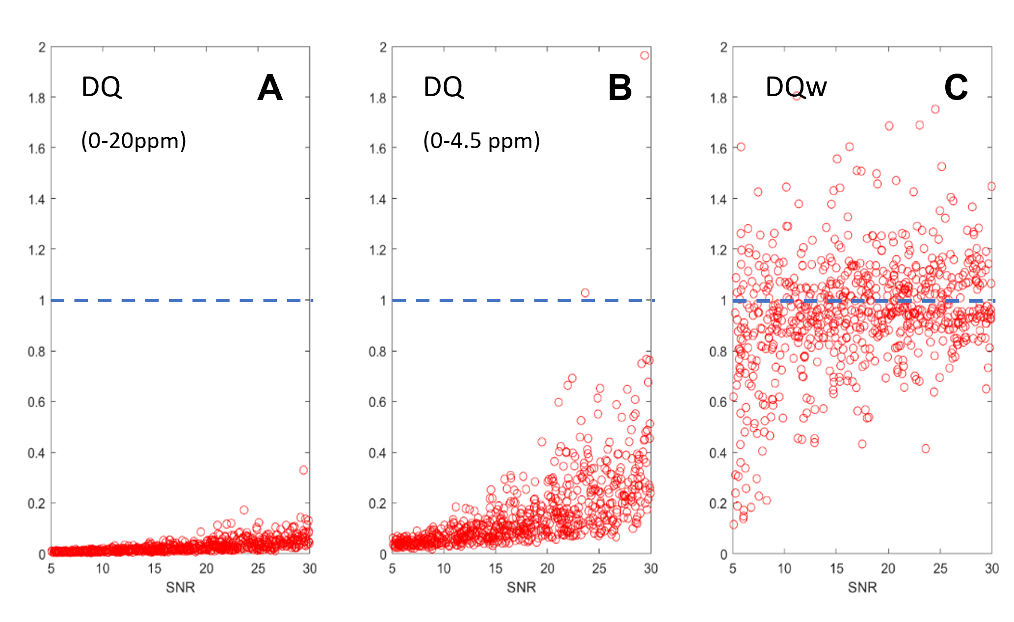
Figure 3.
Efficiency of denoising reflected in denoising quality scores presented as
function of SNR. A) non-weighted DQ
for the full spectral range; B) non-weighted
DQ for the metabolite resonance region; C)
weighted DQw. Mean values are 0.04, 0.24 and 0.97, respectively. Plain DQ
corresponds to a standard error metric and would suggest denoising to be very
effective, while DQw shows that denoising is mostly successful in places where
there are no signals.
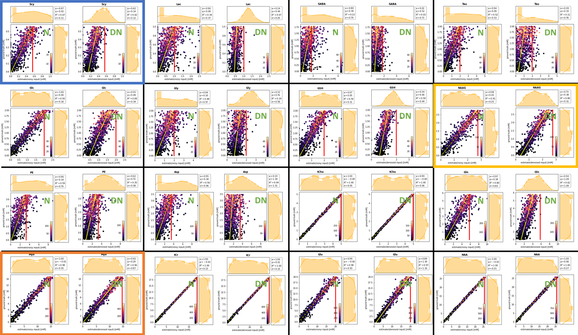
Figure 4.
Illustration of fit results for noisy (N) and denoised (DN) spectra
Plots depict estimated vs. GT concentrations for the whole set.
Projections show distributions for estimates (horizonal) and GT (vertical). Plots
arranged in increasing order of metabolite SNR. Frames highlight examples of low(blue),
medium (yellow) and high (orange) metabolite SNR.
A regression model (y = ax + q; R2)
provides measures to judge how well estimates
represent GT globally. σ is the mean RMSE over
all fits.
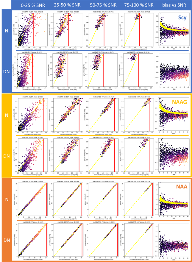
Figure 5.
Illustrative full evaluations for a metabolite with low (blue), moderate
(yellow) and high (orange) metabolite SNR disentangling the effect of noise and
concentration. For each metabolite the correlation of estimates vs. GT was
divided into four groups based on metabolite SNR for noisy and denoised input.
The right column presents the relationship between the overall (water) SNR and
the estimation bias and includes Cramer Rao bounds (yellow dots) for the noisy
case.
DOI: https://doi.org/10.58530/2022/2541