2536
Reducing Artifacts in Readout-Segmented Spectroscopic Imaging at 7T
Amir Seginer1, Graeme A. Keith2, David A. Porter2, and Rita Schmidt3
1Siemens Healthcare Ltd, Rosh Ha'ayin, Israel, 2Institute of Neuroscience and Psychology, University of Glasgow, Glasgow, Scotland, 3Department of Brain Sciences, Weizmann Institute of Science, Rehovot, Israel
1Siemens Healthcare Ltd, Rosh Ha'ayin, Israel, 2Institute of Neuroscience and Psychology, University of Glasgow, Glasgow, Scotland, 3Department of Brain Sciences, Weizmann Institute of Science, Rehovot, Israel
Synopsis
Readout-Segmented COKE (RS-COKE) is an Echo Planar Spectroscopic Imaging (EPSI) variant supporting larger spectral-widths and is therefore useful for spectral imaging at 7T. However, mismatches between the segments at the overlaps lead to artifacts, especially if the lipids signal is not suppressed (to avoid adversely affecting the metabolites signal). We developed a procedure to measure and reduce the readout segment mismatches – through signal and trajectory corrections – leading to improved spectral images and spectra. The procedure was tested by scanning both a special 3D head-shaped phantom – which includes a lipid layer – and human volunteers.
Introduction
RS-COKE (Readout-Segmented COnsistent K-t space Eᴘsɪ)1 is an EPSI (Echo Planar Spectroscopic Imaging) variant offering increased spectral width (SW) and is thus especially promising for spectral imaging of human brain metabolites at 7T. The increased spectral width is achieved both by readout segmentation2 — allowing shorter echo-spacing — and by the COKE scheme3,4 that ensures all same-phase-encode (PE) acquisitions use same-sign readout (RO) gradients — halving the effective dwell time to a single echo-spacing. In practice, COKE switches the N/2 Nyquist ghost artifacts from the temporal domain to the PE domain where they are more benign.RS-COKE is, however, susceptible to image artifacts from mismatches between readout segments. Artifacts are especially pronounced when lipid suppression is off (to avoid adversely affecting the metabolites signal). In this study, we developed a procedure to measure and reduce the RO-segment mismatches, leading to improved spectral images and spectra. Corrections included i) frequency-dependent phase corrections; ii) a correction of the trajectories used by the reconstruction; and iii) a gradual transition between segments to smooth any residual mismatches. The corrections were verified on a special head-mimicking phantom, and on human volunteers.
Methods
Sequence/AcquisitionFigure 1 shows the RS-COKE pulse sequence, implemented on a 7T MAGNETOM Terra (Siemens Healthcare, Erlangen, Germany). It is readout segmented and employs sine-shaped readout gradients. The COKE scheme adds alternating PE blips between the RO gradients, reversing the sign of both PE blips and RO gradients every excitation, to achieve the trajectories shown. A VAPOR water-suppression module is included, as is a refocusing pulse, but no lipid suppression.
The sequence also includes three reference scans on water. The first, a conventional N/2 Nyquist ghost calibration with no PE gradients. Two additional scans, also with no PE gradients, are acquired for calibrating the trajectories. These are acquired at two adjacent RO segments with an additional prepended RO prephaser shifting both segments to overlap around $$$k_x=0$$$, where the signal is maximal. A separate gradient-echo (GRE) scan on water is used to calibrate the complex coil-combination weights per voxel.
Reconstruction
The basic reconstruction steps were:
- Time apodization (exponential with decay constant of 0.1 s).
- Hann filtering of all k-space dimensions.
- Fourier transform (FT) of all dimensions, using regridding along the non-uniformly sampled RO direction.
- An optimized linear coil combination,5 using complex weights derived from the water GRE calibration scan.
Off-Resonance Reconciliation
To resolve off-resonance phase differences along readouts employing opposite gradients, an FT along the time domain was applied (prior to re-gridding) and the linear phase per frequency (and per gradient-sign) was removed. To ensure phase continuity at segment joins, an additional phase — per-segment and per-frequency — was added to each readout.
Segment Trajectory Corrections
The ideal $$$k_x$$$ trajectory of segment $$$s$$$, sampled at time $$$t_n$$$ is given by $$k_x^{(s)}(t_n)=k_{x,\text{ideal}}^{(s=0)}(t_n)+s\cdot\Delta{k}_{\text{seg}},$$ where $$$\Delta{k}_{\text{seg}}$$$ is the $$$k_x$$$ shift between segments. This was replaced by a parametrized trajectory with extra tuning parameters $$$\eta$$$ and $$$\tau$$$ $$k_x^{(s)}(t_n)=\eta\cdot{k}_{x,\text{ideal}}^{(s=0)}(t_n+\tau)+s\cdot\Delta{k}_{\text{seg}}$$ or, for the reference scans (the same with an extra $$$+\Delta{k}_{\text{ref}}$$$ to center the overlap around $$$k_x=0$$$) $$k_x^{(s)}(t_n)=\eta\cdot{k}_{x,\text{ideal}}^{(s=0)}(t_n+\tau)+s\cdot\Delta{k}_{\text{seg}}+\Delta{k}_{\text{ref}}.$$ The parameters $$$\eta$$$ and $$$\tau$$$ were tuned so that odd signals of the trajectory reference scan (acquired during positive gradients) best match at the segments’ overlap — see figure 2. The even trajectories were further updated according to the N/2 Nyquist reference scan. The corrected trajectories were then used in the regridding.
To further reduce artifacts, from residual inter-segment inconsistencies, transitions were also smoothed during the regridding process, effectively averaging the signals with linearly varying weights along the overlap. This was achieved by scaling the regridding sample-weights within the overlap — found for each segment separately — by $$$f$$$ for one segment and $$$(1-f)$$$ for the other, with $$$f$$$ varying along the overlap from 0 to 1; linearly dependent on $$$k_x$$$. See figure 3.
Phantom
A 3D-printed head-shaped phantom designed for 7T was used.5 It included an agar “brain” with metabolites and an oil filled “lipid” layer.
Scan parameters
Scan parameters for the phantom were: TR/TE 2000/14.6 ms, FOV (RO×PE) 200×250 mm2, slice thickness 20 mm, in-plane resolution 4.17×3.9 mm2 (48×64 acquisition matrix), 3 readout segments, SW 2778 Hz, echo spacing 0.360 ms, 294 echoes, and scan duration 6:32 min.
For human imaging the scan parameters were: TR/TE 1600/13 ms, FOV (RO×PE) 260×300 mm2, slice thickness 15 mm, in-plane resolution 4.12×4.69 mm2 (63×64 acquisition matrix), 3 readout segments, SW 2778 Hz, echo spacing 0.360 ms, 638 echoes, and scan duration 5:14 min.
Results
Figure 4 shows phantom results; showing NAA, Cr, and Cho images as well as spectra at two representing points. Results are shown with and without trajectory corrections. Figure 5, shows the same for the human imaging.Discussion & Conclusions
Readout segmented acquisition is prone to artifacts from segment inconsistencies, artifacts are exacerbated by the lipids' strong signal, if lipid suppression is off. These artifacts were reduced by using a reference scan based trajectory correction, smoothing of the signal at segment transitions, as well as — per-frequency and per-segment — phase corrections. The in vivo images still occasionally suffer from some artifacts, which are most likely due to motion and breathing. Full analysis still requires phasing of all data and model fitting of the spectra.Acknowledgements
No acknowledgement found.References
- Keith GA, Seginer A, Porter DA, Schmidt R, Echo-planar spectroscopic imaging with readout-segmented COKE at 7T: Artifact analysis using a purpose-built phantom and simulation. In: Proceedings of the 29th Annual Meeting of ISMRM, 2021.
- Keith GA, Vicari M, Woodward RA, Porter DA, In vivo echo-planar spectroscopic imaging (EPSI) at 7 tesla with readout segmentation for improved spectral bandwidth. In: Proceedings of the 27th Annual Meeting of ISMRM. Montréal, QC, Canada, 2019.
- Webb P, Spielman D, Macovski A. A fast spectroscopic imaging method using a blipped phase encode gradient. Magnetic Resonance in Medicine 1989;12:306–315.
- Schmidt R, Seginer A, Tal A. Combining multiband slice selection with consistent k-t-space epsi for accelerated spectral imaging. Magnetic Resonance in Medicine 2019;82:867–876.
- Jona G, Furman-Haran E, Schmidt R. Realistic head-shaped phantom with brain-mimicking metabolites for 7 t spectroscopy and spectroscopic imaging. NMR in Biomedicine 2021;34:e4421.
Figures
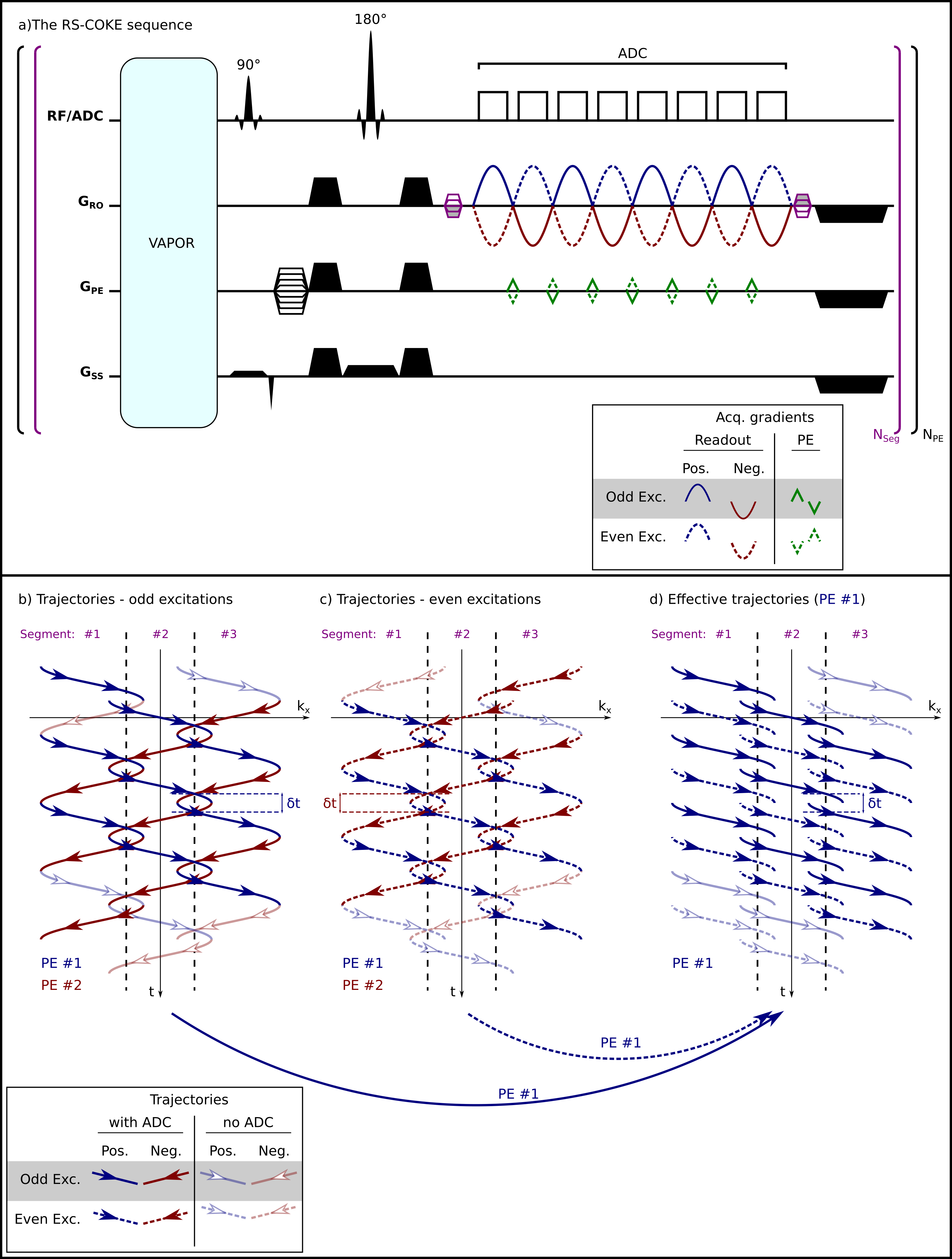
Figure 1: (a) A schematic diagram of the RS-COKE sequence and
(b–d) the resulting $$$k_x$$$-$$$t$$$ trajectories. (b) and (c) are the trajectories
of the odd and even excitations of a 3-segmented RS-COKE. Colors mark different
PEs, “#1” (blue) and “#2” (red). (Faint lines with
hollow arrows mark gradients with data sampling switched off.) All blue
lines (PE #1) can be recombined from (b) and (c) into a consistent set (d) of
acquisitions (same-PE and same-sign gradients). The same is done for PE #2 (not
shown).
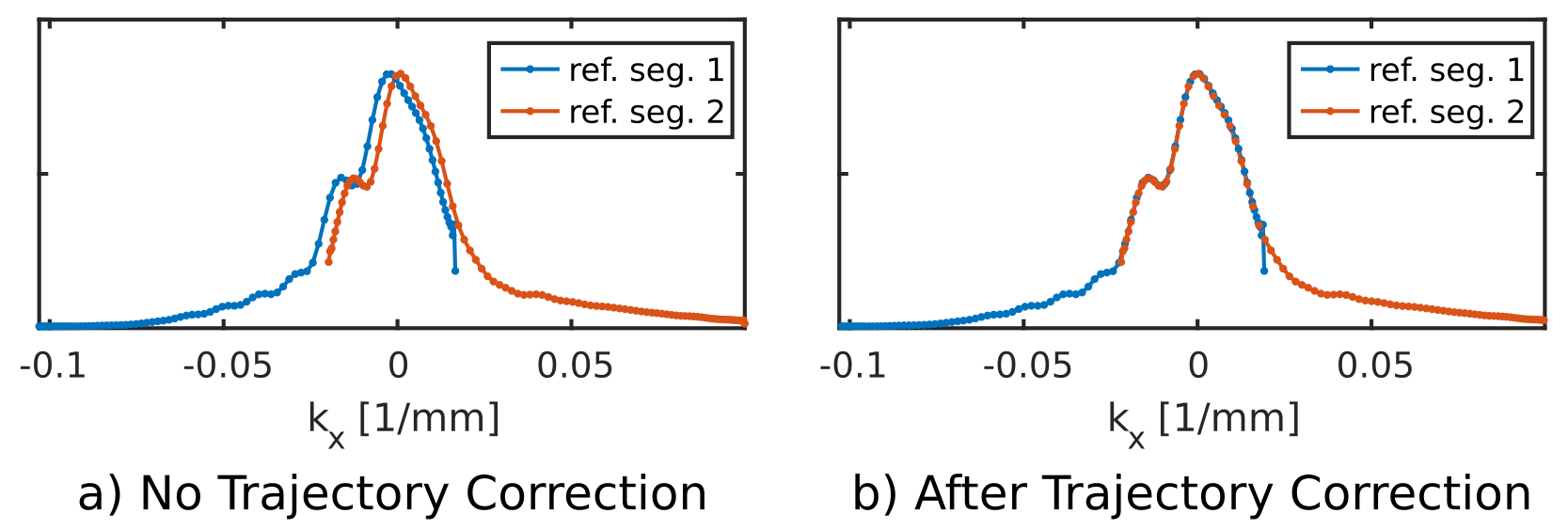
Figure 2: Signals from the trajectory reference scans on
water. Left, before trajectory correction, and right, after. Signals are from
the in vivo scan and are the zero frequency component of the reference scans'
raw data (after apodization and an FT along time).
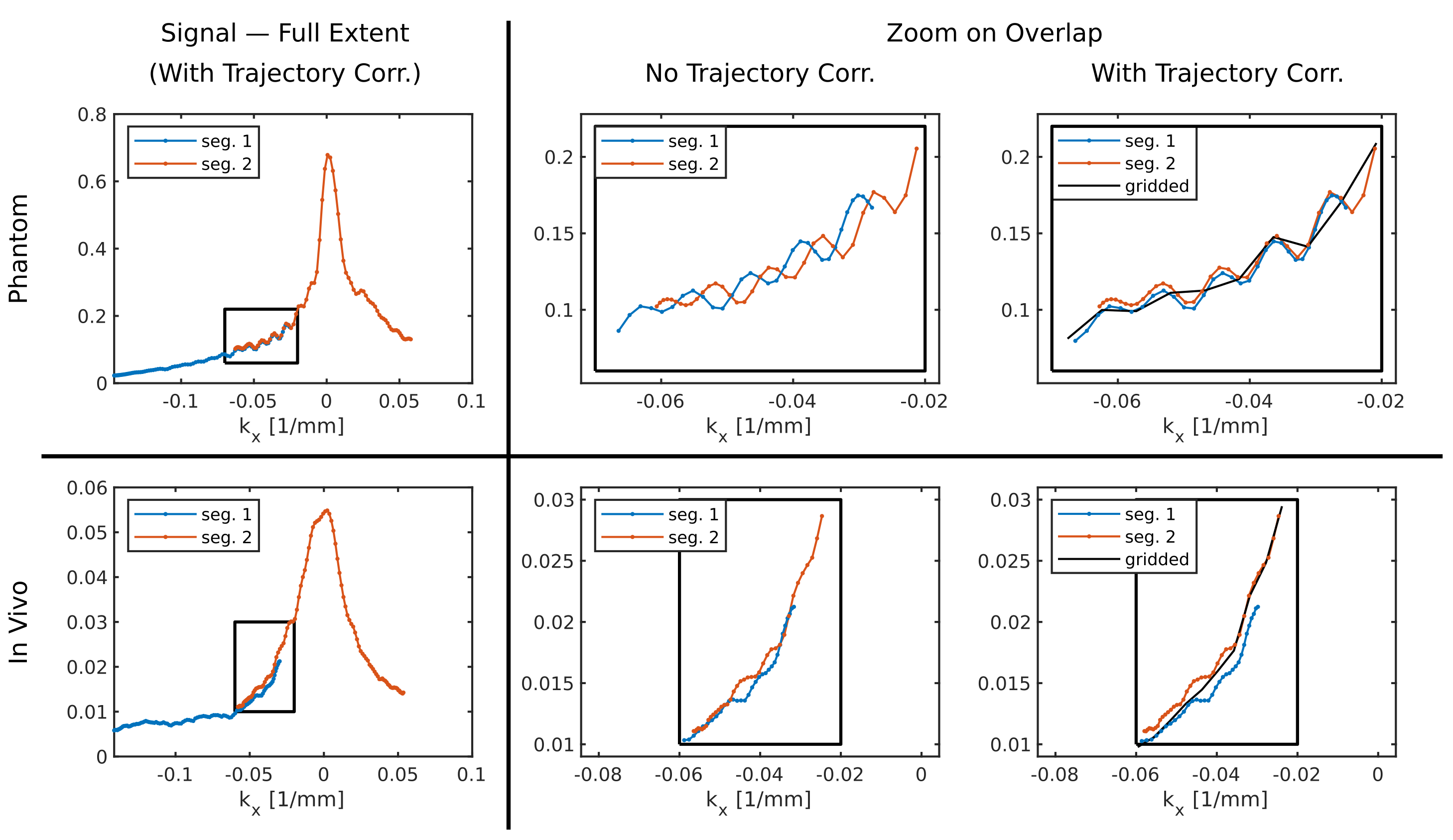
Figure 3: The
effect of the trajectory correction on the signal at the transition between
overlapping segments. Top, phantom example, and bottom, in vivo case. The
signals' full extent is shown to the left, with zooms into the overlap on the
right, both before correction and after (right most). The corrected signals are
overlayed with the gridded signal (black) which smooths the transition — see
main text. After correction, the in vivo signal mismatch is mostly in
amplitude; probably due to physiological changes. Shown are signals at $$$k_y=0$$$ for the
dominant frequency (lipids).
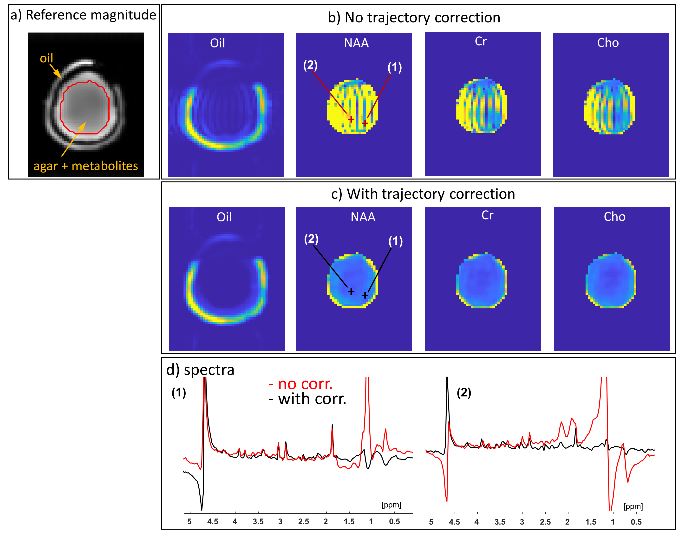
Figure 4: Phantom results. (a) A GRE scan at the slice — used
to calibrate coil combination weights. (b) Spectral images for Lipids, NAA,
Cho, and Cr, without trajectory corrections nor smoothing of transitions. (c)
Same as (b) but with corrections. (d) Spectra at the positions (1) and (2),
marked on the NAA images. Red spectra are without the corrections and black
with. Spectra are the real part after a 3×3 voxel average, while images are
magnitude images after integration. The color range in the lipids images is ×80
that of the metabolites.
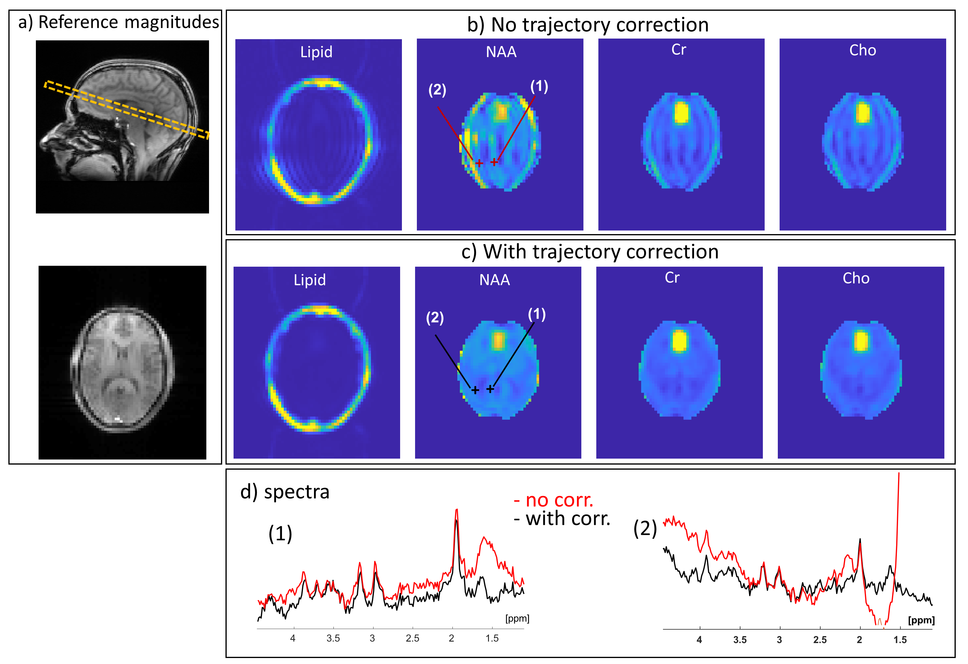
Figure 5: In vivo results. (a) Images for reference; a
localizer showing the slice position and a GRE scan at the slice (with IR for
T1 weighting). (b) Spectral images for Lipids, NAA, Cho, and Cr, without
trajectory corrections nor smoothing of transitions. (c) Same as (b) but with
corrections. (d) Spectra at the positions (1) and (2), marked on the NAA
images. Red spectra are without the corrections and black with. Spectra are the
real part after a 3×3 voxel average, while images are magnitude images after
integration. The color range in the lipids images is ×15 that of the
metabolites.
DOI: https://doi.org/10.58530/2022/2536