Introduction

Complex-valued artificial neural networks (NNs) represent an interesting approach for magnetic resonance imaging (MRI) data, which is inherently complex-valued containing phase information valuable for parameter mapping. Utilizing purely complex operations and architectures, complex-valued NNs have potential to more efficiently process phase information¹. Complex-valued NNs appear especially beneficial for phase sensitive applications like phase reconstruction² or quantitative parameter mapping³, as compared to real-valued NNs. Motivated by recent work proposing to use phase-cycled bSSFP data for simultaneous mapping of relaxation and field parameters with NNs⁴, we further investigate voxelwise multi-parametric tissue characterization using complex-valued NNs. Model training based on complex algebra requires several network modifications to allow for efficient and correct information processing. Therefore, the implementation of different complex hidden layer activation functions is qualitatively compared to the output of known real-valued NNs as well as reference gold-standard relaxometry and field mapping methods.

Methods

3T data of five healthy volunteers were used⁴. 3D sagittal bSSFP data acquired with 12 phase-cycles evenly distributed in the range (0, 2π): φ_j = π/12∙(2j-1), j = 1,2,…12 from four volunteers was used for NN training (isotropic resolution: 1.3x1.3x1.3 mm³, TR/TE = 4.8ms/2.4ms, total acquisition time: 17 min and 13 s). Training data with 6 and 4 phase cycles were retrospectively downsampled. For testing, data acquired in an additional volunteer with a 12-point, 6-point, and 4-point bSSFP acquisition scheme was used, employing in-plane GRAPPA acceleration 2, resulting in a total acquisition time of 10 min 12 s, 5 min 6 s and 3 min 24 s, respectively. Voxelwise phase-cycled bSSFP data was augmented by nearest neighbors in the axial plane, leading to a complex NN input of 108, 54 and 36 voxels (number of phase cycles * 9) for 12, 6 and 4 phase cycles, respectively. The number of input doubles for real-valued NNs as the complex input is separated into real and imaginary parts.

For all volunteers, target T1, T2, B1 and ∆B0 data were acquired with standard reference methods. For T1 and T2, 2D multi-slice IR-SE with variable inversion times and 2D multi-slice single-echo SE with variable echo times was used, respectively. For B1 and ∆B0, TurboFLASH with and without preconditioning RF pulse and standard dual-echo gradient-echo were performed, respectively. For the field map estimates, a median filter was applied to both target and NN output.

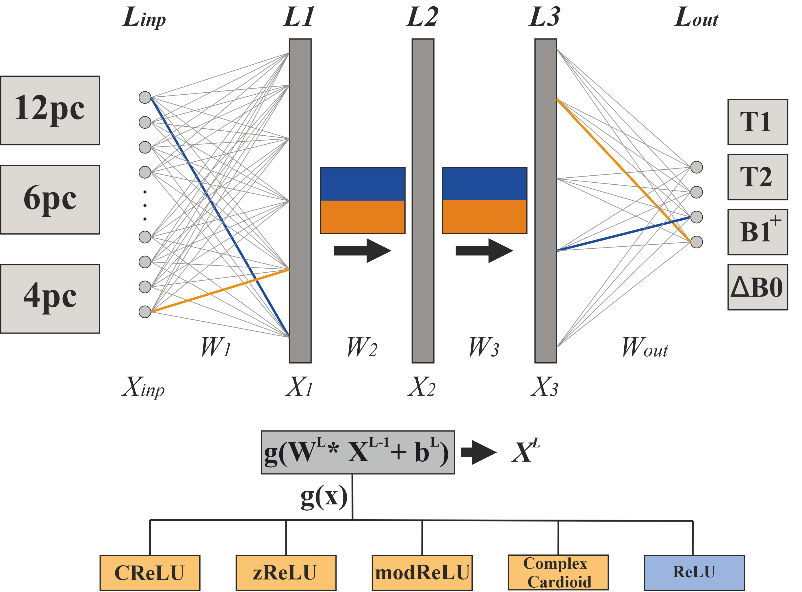
As shown in Figure 1, the forward output for each layer in a fully connected NN model is $$$X^L=g(W^L*X^{L-1}+b^L)$$$, with X^L-1, W^L and b^L referring to the layer input, learnable weight and bias parameters. For the real-valued NNs, the rectified linear unit (ReLU) was used as activation function g(x). However, considering the complex domain with X^L-1, W^L and b^L ∈ ℂ, the ReLU is not feasible. Therefore, a number of different activation functions have been introduced to effectively process complex numbers. For complex-valued NNs, hidden layer activations were performed with the CReLU¹, zReLU¹, modReLU¹, and complex cardioid³ functions. All NNs used a linear activation for the output layer. To enable efficient and direct use of state-of-the-art optimizers and frameworks, the loss function of the complex-valued NNs was defined with the real-valued Euclidean distance³:
$$L=L(y_{pred},y_{tgt})=\frac{1}{2}||y_{pred}-y_{tgt}||^2_2=\frac{1}{2}(y_{pred}-y_{tgt})^H(y_{pred}-y_{tgt})$$

H is known as the transposed complex conjugate. Complex calculations were performed within PyTorch, and the pytorch-complex⁵ package was extended with the complex cardioid activation function. The real-valued NN used the sum of squared error as loss function. NN training processed ~470.000 samples and was trained for 500 epochs, with an early stopping patience of 10. NNs consisted of three hidden layers and 200 or 150 neurons per hidden layer for real- or complex-valued NNs, respectively, to provide a comparable number of learnable parameters for both real- and complex-valued architectures.

Results

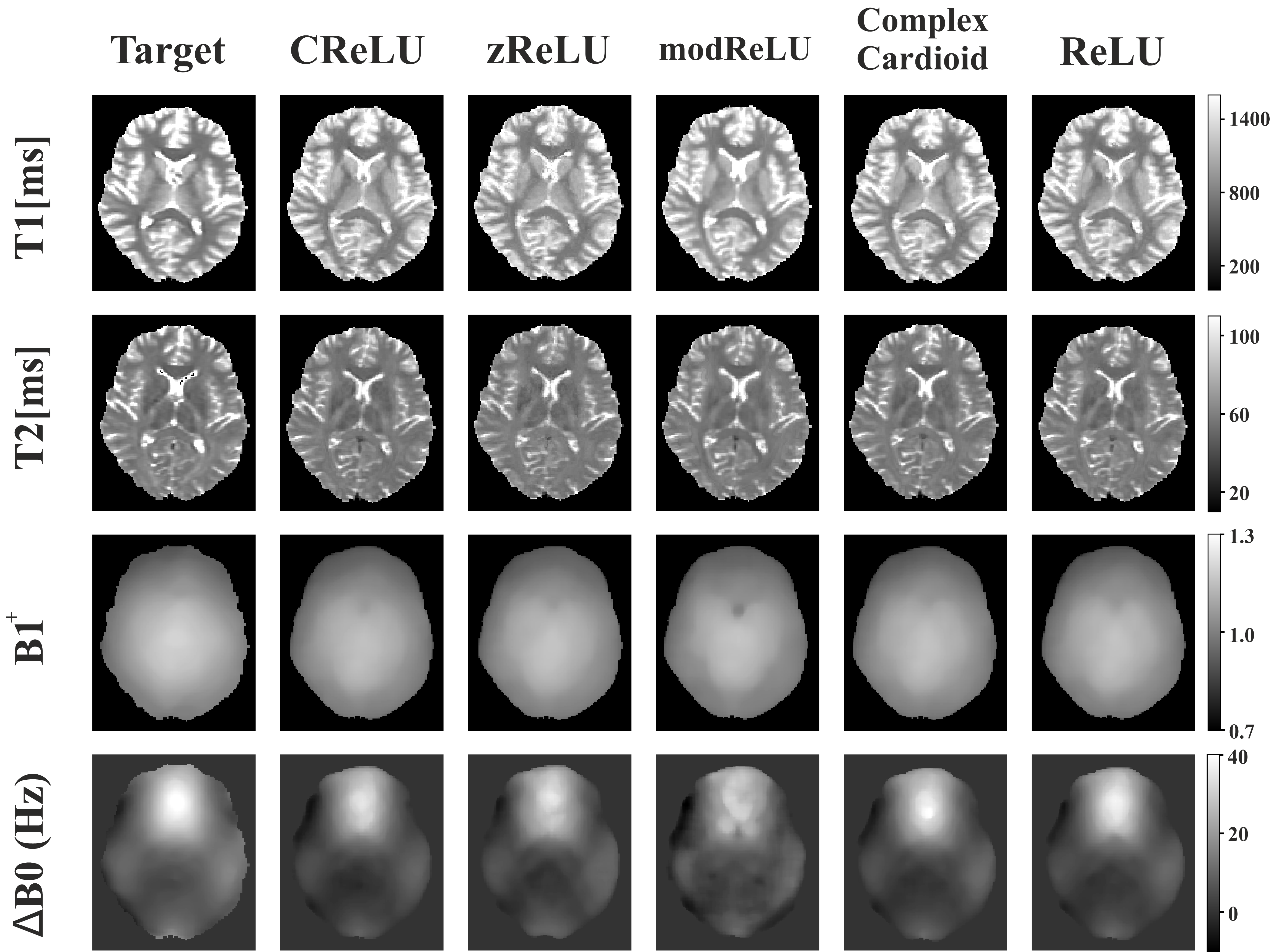
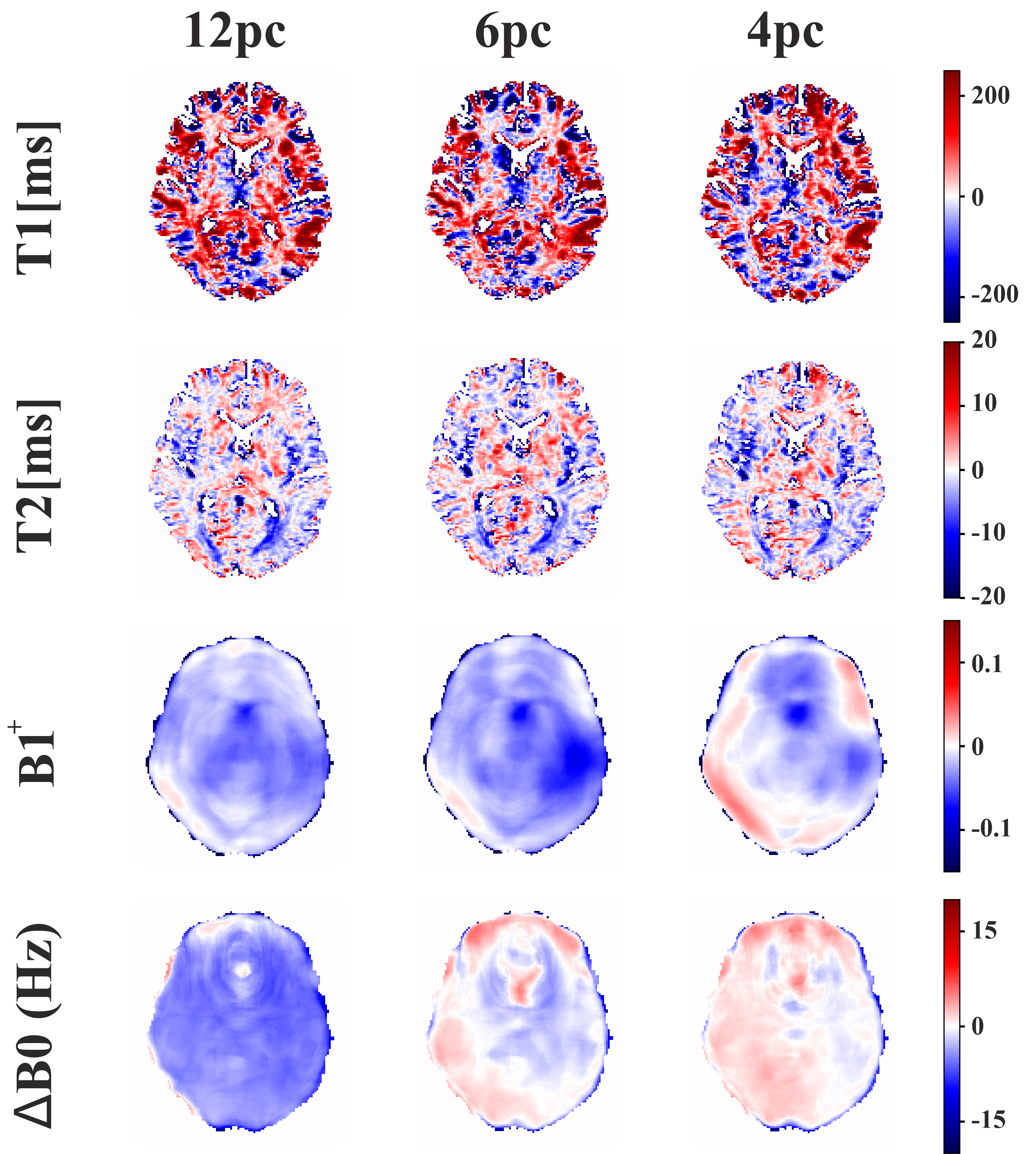
As shown in Figure 2, relaxation parameters and field map estimates of complex-valued NNs are in high agreement with real-valued NNs and the target references. Within T1 and T2 maps of the exemplary axial slice of the testing subject, relevant structures like the putamen or thalamus can be clearly distinguished from surrounding tissue. In comparison to target relaxation maps, zReLU predictions appear noisier and for the field map estimates, ∆B0 is less smooth for modReLU. CReLU and the complex cardioid function show high resemblance with real-valued predictions and target maps.
Error maps for the cardioid complex activation function in Figure 3 display the absolute difference between prediction and target. Low errors can be observed for T2, B1⁺, and ΔB0 for all phase-cycling schemes, while T1 appears to deviate more from the reference. With reduced number of phase-cycles, the model shifts towards a slight overestimation of ∆B0 and B1⁺. T1 and T2 error maps show overestimations in white matter and underestimation in gray matter structures, while preserving comparable performance for all phase-cycles.

Discussion and Conclusion

Complex NNs present an alternative to already known real-based NN models for quantitative imaging. The natural representation of real and imaginary components in complex numbers could facilitate a more effective processing of relevant phase information with a smaller amount of data or smaller architectures. In future, we will investigate in-depth in which settings the increased phase sensitivity of complex-valued NNs yields an improvement in accuracy or precision of the predicted parameters over real-valued architectures.

Acknowledgements

No acknowledgement found.

References

1. Trabelsi C, Bilaniuk O, Zhang Y, et al. Deep Complex Networks. ArXiv170509792 Cs. Published online February 25, 2018. Accessed November 6, 2021. http://arxiv.org/abs/1705.09792

2. Cole E, Cheng J, Pauly J, Vasanawala S. Analysis of deep complex‐valued convolutional neural networks for MRI reconstruction and phase‐focused applications. Magn Reson Med. 2021;86(2):1093-1109. doi:10.1002/mrm.28733

3. Virtue P, Yu SX, Lustig M. Better than real: Complex-valued neural nets for MRI fingerprinting. In: 2017 IEEE International Conference on Image Processing (ICIP). IEEE; 2017:3953-3957. doi:10.1109/ICIP.2017.8297024

4. Heule R, Bause J, Pusterla O, Scheffler K. Multi‐parametric artificial neural network fitting of phase‐cycled balanced steady‐state free precession data. Magn Reson Med. 2020;84(6):2981-2993. doi:10.1002/mrm.28325

5. Chatterjee S, Sarasaen C, Sciarra A, et al. Going beyond the image space: undersampled MRI reconstruction directly in the k-space using a complex valued residual neural network. In: 2021 ISMRM & SMRT Annual Meeting & Exhibition. May 2021.