2526
Improved detection of multiple kidney pH compartments by deep learning in MRS and MRSI with hyperpolarized 13C-labelled zymonic acid1Department of Nuclear Medicine, TUM School of Medicine, Klinikum rechts der Isar, Technical University of Munich, Munich, Germany, 2Department of Informatics, Technical University of Munich, Munich, Germany
Synopsis
Accurate determination of peak position is challenging for spectra with dense spectral regions paired with low SNR as occuring in pH measurements using hyperpolarized [1,5-13C2,3,6,6,6-D4]zymonic acid in kidney of mice. Despite scarcity of available data from preclinical experiments, convolutional neural networks (CNN) and multilayer perceptrons (MLP) could be trained by complementing real and augmented data with synthetic spectra. While MLPs do not achieve suitable performance, CNNs predict pH compartments with an accuracy comparable or superior to supervised line fitting in synthetic test spectra. Further, CNNs allow generation of composite pH maps with improved quality while quantitatively agreeing with line-fitted maps.
Introduction
Quantification of pH using hyperpolarized (HP) MRI is often done via peak position analysis of the chemical shift of pH-sensitive molecules1. Typically, spectra are fitted via an optimization procedure returning peak positions and amplitudes. However, such line fitting procedures are error-prone in cases of low signal-to-noise ratio (SNR) and peak overlap, e.g. for multiple pH compartments within kidneys2. Deep learning has shown its potential for magnetic resonance spectroscopy (MRS) and -imaging (MRSI) data in several applications to improve analysis of noisy data with interfering signals3,4, however often requiring large amounts of training data. In this work, we investigate whether deep learning can improve the prediction of multiple pH compartments for pH mapping based on hyperpolarized (HP) MRSI data of [1,5-13C2,3,6,6,6‑D4]zymonic acid (ZA) which are for ethical reasons only scarcely available in preclinical experiments.Methods
HP: 27 mg ZA and 25 mg 13C-urea were co-polarized using a HyperSense hyperpolarizer and dissolved in TRIS-buffered D2O.Hardware: MR-experiments were performed in a 7 T small animal scanner and a 31 mm 13C/1H-volume resonator.
HP MRSI/MRI: HP acquisitions were performed in seven C57BL/6 mice. FIDCSI used FA 15°, matrix size 14x12, slice thickness 5 mm, FOV 28x24 mm2, bandwidth 3201 Hz, 256 points. PRESS used total echo time 13.9 ms, FA 90°-180°-180°, bandwidth 2000-3201 Hz, 1024 points, voxel size 5×5×7 mm.
Line Fitting + Manual analysis: ZA- and urea peaks were identified by a peak picking algorithm in MatLab. Line fitting used a linear combination of Lorentzians: $$y(pH)=\displaystyle\sum_{i=1}^{N}\frac{a_i\cdot w_i^2}{w_i^2+[x+ZA_i(pH)]^2}$$
with a pH calibration curve ZAi2. Spectral fits were visually inspected to assess peak detection and pH fitting. CSI data was segmented into spectra containing three compartments (Fig. 4b, white) or less than three pH compartments.
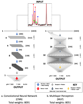
Network training and datasets: Convolutional neural networks (CNN) and multilayer perceptrons (MLP) were designed (Fig. 1) and implemented in Keras. Synthetic spectra Xs were generated according to:
$$X_s=b_0+\epsilon+S\cdot y(pH)$$
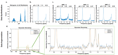
from a model spectrum y(pH), baseline b0, noise ε and SNR S. Fig. 2a shows the distribution of pH compartments for synthetic spectra derived from HP ZA-MRSI5. B0 inhomogeneities and shim variations were accounted for by varying linewidths, amplitudes and absolute peak positions to generate basic spectra (Fig. 2b). Hardware, perfusion and polarization variations were accounted for by adding Gaussian noise addition with SNRs 2–7 (Fig. 2c). 10020 synthetic spectra were generated (training: 10000, testing: 20) and complemented by 40 augmented spectra for training generated by Gaussian denoising (Fig. 2d) from 8 real spectra. Network optimization used NADAM6 (batch size: 200, epochs: 400) either with synthetic spectra (CNNsyn/MLPsyn) or a mix of augmented and synthetic data (CNNmix/MLPmix). CNNmix and line fitting were further tested on CSI datasets for composite pH mapping.
pH mapping: pH maps were generated by voxel-wise averaging of pH compartments obtained from line fitting or CNN predictions and interpolated by a factor of four. CNN predictions were performed for voxels containing three pH compartments as detected by visual inspection (Fig. 4b).
Results
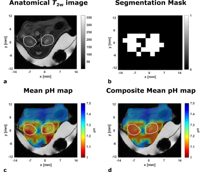
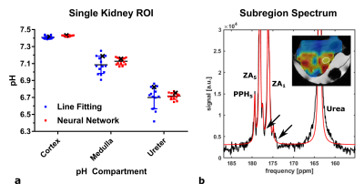
Supervised line fitting and four different networks trained on 20 synthetic spectra were compared and the results are visualized by Bland-Altman-plots (Fig. 3). Line fitting reveals systematic underestimation of the cortex pH and highest uncertainty for the medulla. CNNs show good accuracy for all compartments with best performance for the cortex. Overall, MLPs show poor performance with uncertainties up to 0.25 pH units. No considerable difference between performance for different training datasets is observed. pH mapping for mouse kidneys (Fig. 4a) using line fitting only (Fig. 4c) or a composite pH map (Fig. 4d), involving a segmentation mask (Fig. 4b), which combines CNN predictions and line fitting, shows good qualitative agreement regarding absolute pH values while composite maps appear more homogeneous. pH compartments for single kidneys (n=14) indicate good agreement between pH compartments obtained from manual maps (pHcortex=7.41±0.02, pHmedulla=7.09±0.10, pHureter=6.70±0.13) and composite maps (pHcortex=7.43±0.01, pHmedulla=7.13±0.05, pHureter=6.72±0.04)(Fig. 5a) which also agrees with literature values2,7. Line-fitted pH map heterogeneity (Fig. 4c) might be related to poor fitting of low-SNR-compartments as indicated by ROI spectra from heterogeneous regions (Fig. 5b).Discussion
Here, CNNs outperform MLPs in predicting three pH compartments in synthetic kidney test data. In comparison, CNNs show better accuracy and less uncertainty. Further, pH maps composed from CNN predictions and line fitting show better intra- and inter-kidney agreement regarding pH (Fig. 5) which we assume to be consistent with actual renal pH values in healthy subjects. Neural networks usually require large amounts of training data. However, generating larger datasets is challenging for preclinical studies, especially for HP 13C-MRSI with demanding experimental setups. However, this work demonstrates the feasibility to train networks on a limited amount of real data whilst most of the training data were synthetically generated based on a spectral model.Conclusion
Neural networks were evaluated for prediction of pH compartments from acquisitions of HP ZA in mouse kidney. CNNs achieve the best results and outperform supervised line fitting. Thus, small amounts of experimental data combined with suitable networks and training allows fast and reliable evaluation of HP MRS(I) data and generation of composite pH maps from line fitting and CNN predictions. This approach can also be extended to other organs, tumors and varying numbers of pH compartments.Acknowledgements
We acknowledge support from Dr. Geoffrey J. Topping for help with setting up hyperpolarized 13C acquisition protocols. Further, we acknowledge support from Dr. Christian Hundshammer for help with zymonic acid polarization and synthesis and help from Sandra Sühnel with animal experiments.
This research was funded by the Deutsche Forschungsgemeinschaft (DFG, German Research Foundation, Sonderforschungsbereich (SFB) 824, subprojects A7 and Z3, grant number 391523415), the Young Academy of the Bavarian Academy of Sciences and Humanities and the European Union’s Horizon 2020 research and innovation program under grant agreement No 820374.
References
1. Anemone A, Consolino L, Arena F, et al. Imaging tumor acidosis: a survey of the available techniques for mapping in vivo tumor pH. Cancer Metastatis Rev. 2019;38(1-2): 25-49.
2. Düwel S, Hundshammer C, Gersch M, et al. Imaging of pH in vivo using hyperpolarized 13C-labelled zymonic acid. Nat Commun 2017, 8, 15126, doi: 10.1038/ncomms15126.
3. Chen D, Wang Z, Guo D, et al. Review and Prospect: Deep Learning in Nuclear Magnetic Resonance Spectroscopy. Chemistry 2020, 26, 10391-10401.
4. Das D, Coello E, Schulte R F, et al. Quantification of Metabolites in Magnetic Resonance Spectroscopic Imaging Using Machine Learning. In Medical Image Computing and Computer Assisted Intervention - MICCAI 2017 2017; 462-470.
5. Grashei M, Suehnel S, Topping G J, et al. Multi-compartment pH detection in healthy and tumour bearing mice using hyperpolarized deuterated [1,5-13C2]zymonic acid. Digital Poster at ISMRM2020 International Conference 2020.
6. Dozat T. Incorporating Nesterov Momentum Into Adam. In Proceedings of International Conference on Learning Representations 2016 - Workshop Track.
7. Raghunand N, Howison C, Sherry A D, et al. Renal and Systemic pH Imaging by Contrast-Enhanced MRI, Magn Reson Med. (2003); 49: 249 – 257.
Figures

Neural network architecture for the (a) CNN and the (b) MLP. Both networks consist of 4 feature extraction layers, for which they learnt a mapping between the input spectra and multiple pH compartments. The length of the spectrum or feature maps, which are used as the input to each next convolutional or dense layer, are shown in the square brackets.
a: The number of filters is 4, 4, 8, and 8. Round brackets indicate convolutional kernel sizes.
b: The number of neurons is 16, 16, 32, and 32. Dense layers are represented with half (MLP) or quarter (CNN) the number of nodes, except for output layers.

Synthesis of three pH compartment spectra for CNN- and MLP-training.
a: Normal distributions of pH values for pH compartments to generate synthetic spectra.
b: Example spectrum containing 3 pH compartments without added noise.
c: Addition of noise to obtain synthetic spectra with minimal SNR between 2 and 7 (SNR 2, 5, and 7 are shown exemplarily).
d: Exemplary spectra for five-scale Gaussian denoising to increase the real training data size. Only the first and the fifth scale-denoised spectra and an enlarged version of the spectra (green box) are shown.


a: Axial anatomical T2w image of mouse kidneys (white ROIs).
b: Segmentation mask for a hyperpolarized [1,5-13C2]zymonic acid CSI acquisition. White areas indicate voxels which contain three pH compartments as detected by voxel-wise spectra inspection and supervised line fitting.
c: Mean pH map based on voxel-wise averaging of all pH compartments being detected by manual line fitting.
d: Composite mean pH map generated from voxel-wise averaging of pH compartments. For regions with positive mask (b), pH compartments and mean pH values are obtained from CNN predictions.

a: pH Compartments derived from single kidney ROIs in pH maps generated from line fitting and composite pH maps generated from line fitting and CNN predictions as shown in Fig. 4c, d. Mean pH values of kidney compartments from both pH maps show good agreement while neural networks show less variation for pH compartment values. pH values from the kidney marked in the inset of b are indicated with a black cross.
b: ROI spectrum from region drawn in inset image (white ROI). Arrows indicate where line fitting is incomplete due to low SNR, resulting in the observed map heterogeneity in Fig. 4c.