2523
Prior-knowledge MRS Metabolite Quantification using Deep Learning Frameworks: A proof-of-concept1SCAN, Institute of Diagnostic and Interventional Neuroradiology, Bern, Switzerland
Synopsis
We implemented a mathematical representation of a prior-knowledge model in a Neural Network using a Tensorflow. The trainables tensors are directly the free parameters of the model and we do metabolite quantification by overfitting the output to the signal that we want to replicate. We found that this way of fitting has a relatively low performance in time domain but similar to the state-of-the-art (TDFDFit) when using frequency domain. In addition we have a faster method and it can be used in future works as a component of a more complex network.
Introduction
Current deep-learning (DL) implementations have shown to be a fast method for MRS-metabolite-quantification1-3. However, these implementations do not ensure that their predictions are always reliable or precise, which is mandatory for methods being applied to clinical data. Here we propose to implement a prior-knowledge fitting model using Tensorflow4, aiming at finetuning the initial seeds predicted by DL until optimal convergence. A similar architecture for a different purpose was implemented3 for three Voigt-lines (NAA;Cho;Cr). Our approach uses prior-knowledge to maximally lower the model dimensionality and allows a flexible number of metabolites. The implementation was tested the 14 in vivo MRSI-datasets. We compare the performance when fitting in time-domain (TD) and frequency-domain (FD) against the results obtained with the TDFDFit-algorithm5.Methods
Prior Knowledge Model: We defined a fitting model using 9 metabolites (Cho, Glu, Lac, Gln, Cre, Asp, NAA(2.01ppm), NAA(2.4ppm), and Myo-Inositol). The model consisted of 12 free parameters (9 amplitudes, one-common-phase, one-common-frequency-shift, and one-common-Lorentzian-width). Each metabolite was simulated using NMRScope-B6 and the full prior-knowledge model was defined using SpectrIm-QMRS7. The final model for a sum-signal can be represented as:$$S(\omega) = FFT(\:e^{-W_c\,x(t)+i\,(\omega_c\,x(t)\,+\,\phi_c)}\sum^9_{i=1}A_i\,M_i(t)\,e^{i\,\Delta\omega_i\,x(t)}\:)\:\qquad\qquad(Eq.1)$$ where $$$A_i$$$ is the amplitude of each metabolite, $$$x(t)$$$ a time vector, $$$\Delta\omega_i$$$ is a fixed prior-knowledge, $$$M_i(t)$$$ the simulated metabolite basis, and $$$W_c$$$, $$$\phi_c$$$ and $$$\omega_c$$$ are the common-width change, common-phase change and common-frequency-shift change respectively.Clinical dataset: We tested the network performance on 14 in-vivo 2D-MRSI-datasets (total 1712 spectra, B0=3T, semiLASER, TE=135ms). Both TD and FD signals were used to test and compare the performance of the algorithms.
Pre-processing: The pre-processing consisted of water removal and offset correction in FD. The prior-knowledge model, defined by (Eq.1), was fitted using TDFDFit and is regarded as ground-truth. All pre-processing/visualization of datasets/results were done with SpectrIm-QMRS.
Neural Network: The model defined by (Eq.1) has been implemented as a Neural-Network (NN), using Tensorflow. Since all mathematical operations in this model are differentiable, we can backpropagate through the network and overfit the trainable-tensors which are the 12 parameters of the model.
In this approach, the network output (all complex-typed signals) should resemble the original signal as well as possible. On the other hand, the inputs of the networks are all the simulated metabolite-basis, a time vector, and a constant tensor that multiply each trainable parameter. In Figure 1 we show a representation of the network, with and without the FFT-layer for fitting in FD and TD respectively.
The implementation can simultaneously generate n spectra, and fit the 12*n parameters. Given the fact that tensorial operations are optimized for GPU, this results in a computation-time reduction compared to serial NN-fitting. As a metric for the goodness of the fitting, we use the Mean-Squared-Error function(Loss) of the spectra normalized to the noise level.
Results
First, we fitted the datasets by TDFDFit which results are considered as ground-truth. Then we fitted with the network for both TD and FD. The NN-fitting was performed in an Nvidia GTX 1060 - 6GB, using an Adam-optimizer with a learning rate of 0.1.For the parameters, Figure 2 displays scatterplots of fitting in TD and FD. Horizontally displayed the TDFDFit-results, vertically the NN-results. We observed that using FD not only the intense metabolite does have a small dispersion (variance), but also the non-intense metabolites, which are relatively more affected by the noise, and also have a small dispersion.
On the other hand, using TD for fitting, we found that the NN does fit a smaller amplitude consistently, and also observed the same behavior for the common-Lorentzian-width. An explanation could be the higher complexity of the Loss in TD since all metabolites are overlapping with each other. The convergence seems to be reaching a local minimum.
In Table 1 we present the percentage error for both TD and FD compared to TDFDFit. As expected, the relative error in the principal metabolites (Choline, Creatine, NAA(2.01)) are smaller since they contribute mostly to the Loss and are less sensitive to the noise level.
We also investigated the distribution of Loss of the network relative to the Loss obtained with TDFDFit. Figure 3 shows that in FD our fitting is practically spoken identical to TDFDFit, giving 40% of the time a slightly better fit, and the TDFDFit-loss is on average 0.2% better. On the other hand, in TD we found that our fitting is, on average, 68% worse than TDFDFit.
In Figure 4 we show all parameter maps for one in vivo 2D-MRSI-dataset.
Discusion
We implemented an NN-scheme for prior-knowledge model-fitting of in-vivo MRSI-data with a variable number of metabolites. We have proven that it is a viable option compared to state-of-the-art NLLS-fitting. Our NN approach is not only faster, given the high optimization level of Tensorflow, but the work presented here can be regarded as a proof-of-concept that these NN-architectures also perform excellently for more complex models.In order to investigate the precision, we plan the following: firstly a Neural Network could be trained to predict an initial seed, and secondly, the overfitting approach, as presented here, is performed to enable the verification that the results are also reliable. Since the predicted initial seed will be usually close to the real value, the convergence should be fast.
Acknowledgements
The project leading to this application has received funding from the European Union's Horizon 2020 research and innovation programme under the Marie Sklodowska-Curie grant agreement No 813120References
1) Hatami, N., Sdika, M., & Ratiney, H. (2018, September). Magnetic resonance spectroscopy quantification using deep learning. In International Conference on Medical Image Computing and Computer-Assisted Intervention (pp. 467-475). Springer, Cham.
2) Lee, H. H., & Kim, H. (2019). Intact metabolite spectrum mining by deep learning in proton magnetic resonance spectroscopy of the brain. Magnetic resonance in medicine, 82(1), 33-48.
3) Gurbani, S. S., Sheriff, S., Maudsley, A. A., Shim, H., & Cooper, L. A. (2019). Incorporation of a spectral model in a convolutional neural network for accelerated spectral fitting. Magnetic resonance in medicine, 81(5), 3346-3357.
4)M. Abadi, P. Barham, J. Chen, Z. Chen, A. Davis, J. Dean, M. Devin, S. Ghemawat, G. Irving, M. Isard, et al., Tensorflow: A system for large-scale machine learning (2016), https://doi.org/10.5281/zenodo.5043456. Software available from tensorflow.org.
5) Slotboom, J., Boesch, C., & Kreis, R. (1998). Versatile frequency domain fitting using time domain models and prior knowledge. Magnetic resonance in medicine, 39(6), 899-911.
6) Starčuk Z Jr, Starčuková J. Quantum-mechanical simulations for in vivo MR spectroscopy: Principles and possibilities demonstrated with the program NMRScopeB. Anal Biochem. 2017; 15;529:79-97.
7) Pedrosa de Barros, N., McKinley, R., Knecht, U., Wiest, R., & Slotboom, J. (2016). Automatic quality control in clinical 1H MRSI of brain cancer. NMR in Biomedicine, 29(5), 563-575.
Figures
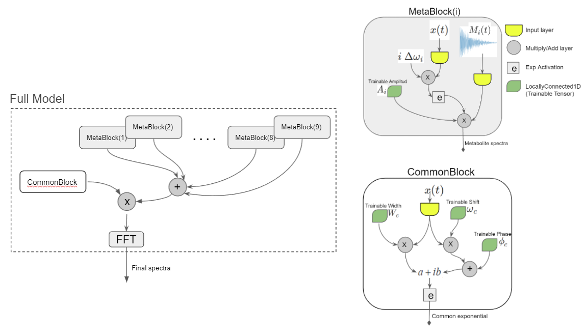
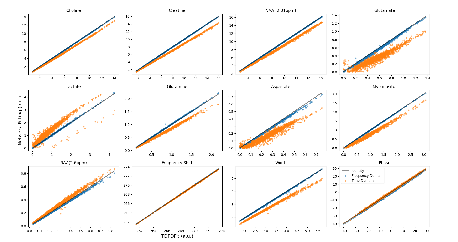
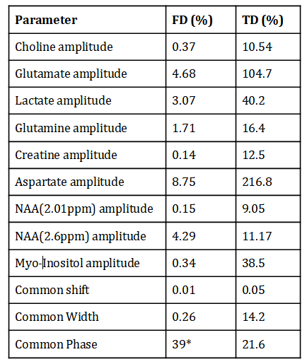
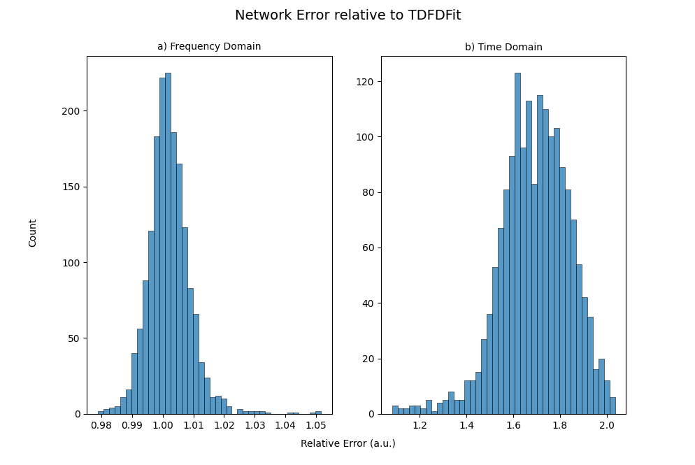
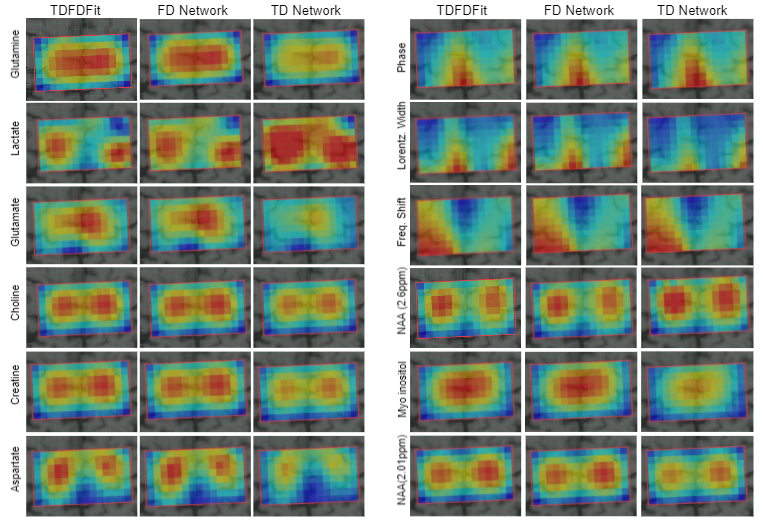
Figure 4: Map of metabolite concentration and common width, phase, and frequency shift for the three methods. In columns each fitting method and in rows the corresponding parameter. Clearly, differences between the ground-truth and TD network fitting can be seen.