2516
3D magnetic resonance fingerprinting at 50 mT with integrated estimation and correction of image distortions due to B0 inhomogeneities
Thomas O'Reilly1, Peter Börnert2, Andrew Webb1, and Kirsten Koolstra1
1Leiden University Medical Center, Leiden, Netherlands, 2Philips Research Hamburg, Hamburg, Germany
1Leiden University Medical Center, Leiden, Netherlands, 2Philips Research Hamburg, Hamburg, Germany
Synopsis
Strong B0 inhomogeneities in compact point-of-care low field permanent magnet systems can cause image distortions and reduced signal for large field-of-view images. MRF, as a flexible acquisition framework, can encode these effects into the acquisition process, to incorporate them into the reconstruction process. In this work, we use an alternating TE in the MRF sequence that supports ΔB0 estimation and image distortion correction of the MRF data. This method reduces distortions in the relaxation time maps without needing to acquire an additional ΔB0 map.
Introduction
Magnetic resonance fingerprinting (MRF) offers a way to acquire relaxation time maps in an efficient manner and has shown its use in many 1.5T and 3T applications1. The T1 and T2 relaxation times can potentially be used to generate a variety of image contrasts retrospectively2. This could be particularly relevant at low field3, where scans take many minutes due to a lower signal-to-noise ratio (SNR). Portable point-of-care permanent magnet systems often have large B0 inhomogeneities, which can cause image distortions and signal dropout. MRF is a flexible acquisition framework4 that can encode the B0 field inhomogeneities in the acquisition process, to incorporate them in the reconstruction process. In this work, we use an alternating TE pattern in the MRF sequence that supports ΔB0 estimation from the MRF data. We use the reconstructed ΔB0 map to correct for B0-induced image distortions of the MRF images, before matching them to the calculated dictionary. This method reduces distortions in the relaxation time maps without needing to acquire an additional ΔB0 map.Methods
Hardware: We used a 50 mT Halbach magnet consisting of 23 rings filled with neodymium boron iron magnets, shown in Fig. 1A, with custom-built RF and gradient amplifiers and a Magritek Kea2 spectrometer (Fig. 1B). A 15 cm diameter, 15 cm long solenoid coil was used in transceive mode (Fig. 1C). A mechanical robot with a magnetic field probe was used to map the B0 field during system installation.Fingerprinting implementation: MRF data were acquired with a FISP sequence5, using an optimized flip angle pattern of 240 RF shots, a constant TR of 12 ms and an alternating TE pattern to support ΔB0 estimation, shown in Fig. 2A. The dictionary was generated using the extended phase graph formalism, with T1 values ranging from 20-500 ms (5 ms steps), T2 values ranging from 10-500 ms (5 ms steps) and B1+ fraction ranging from 0.05-1.50 (0.05 steps).
MR Data acquisition: Experiments were performed in the lower leg of 2 healthy volunteers with informed consent obtained. Three-dimensional MRF scans were acquired with a Cartesian sampling scheme shown in Fig. 2B. Scan parameters: FOV = 170×150×99 mm3, resolution = 2.5×2.5×3.0 mm3, TE1/TE2/TR = 6.00/6.15/12.0 ms, imaging bandwidth (BW) = 294 Hz/pixel, undersampling factor = 8.6, scan time = 13 min and 6 s. Inversion recovery (inversion times = 25/50/75/100/150/300 ms) and multi-echo-spin-echo (TEs = 20/40/60/80/100/120/140/160/180/200 ms) were used for reference T1 and T2 mapping, respectively. A TSE-based ΔB0 map was acquired for comparison6.
Reconstruction: MRF images were reconstructed using a matrix completion-based reconstruction on the two separate TE series7. A ΔB0 map was estimated from the two series using total variation regularization and spherical harmonic decomposition and used in a model-based reconstruction framework to correct for image distortions6. The resulting combined image series were matched to the dictionary using the simulated B1+ excitation profile (Fig. 1E) as prior information for each slice. This pipeline is schematically shown in Fig. 2C.
Results
Figure 3 shows that the relaxation times obtained with MRF (constant TE, without distortion correction) are close to those obtained with the reference techniques, but the SNR of the MRF maps is lower compared to that of the reference maps, as expected. Using an alternating TE pattern results in very similar parameter maps compared to using a constant TE (both without distortion correction), as shown in Fig. 4. Estimating a ΔB0 map from the alternating TE pattern and using it in a model-based MRF reconstruction results in matched parameter maps with reduced distortions. The estimated ΔB0 map is in the same range as that estimated from a TSE sequence, with a maximum error of 105 Hz.Discussion
The acquired MRF ΔB0 map corresponds with the map measured with a robot and that measured with a fully encoded TSE sequence. The difference between the MRF-based ΔB0 map and the TSE-based ΔB0 map could have been introduced by hardware imperfections (spectrometer timing jitter, eddy currents, etc.) leading to phase errors in the MRF sequence or by heating of the magnet during the imaging session. Using the ΔB0 map in a model-based reconstruction framework reduces the image distortions along the readout direction of the parameter maps. The remaining signal void at the left side of the M0 map is a result of through-plane B0-induced dephasing, for which the current reconstruction algorithm does not correct. Future work could resolve this by incorporating a ΔB0 map with a higher through-plane resolution into the signal model.Conclusion
It is possible to integrate ΔB0 estimation and correction in an MRF acquisition and reconstruction framework for a 50 mT permanent magnet MR system. The proposed framework reduces the image distortions of the MRF relaxation time maps without increasing the scan time.Acknowledgements
This work is supported by the following grants: Horizon 2020 ERC FET-OPEN 737180 Histo MRI, Horizon 2020 ERC Advanced NOMA-MRI 670629, Simon Stevin Meester Award and NWO WOTRO Joint SDG Research Programme W 07.303.101. We would also like to thank Hanna Liu for sharing the optimized flip angle train with us.References
1. Panda, Ananya, et al. "Magnetic resonance fingerprinting–an overview." Current opinion in biomedical engineering (2017) 3:56-66.
2. Blystad, Ida, et al. "Synthetic MRI of the brain in a clinical setting." Acta radiologica (2012) 53(10): 1158-1163.
3. O’Reilly, Thomas, and Andrew G. Webb. "In vivo T1 and T2 relaxation time maps of brain tissue, skeletal muscle, and lipid measured in healthy volunteers at 50 mT." Magnetic Resonance in Medicine (2021).
4. Sarracanie, Mathieu. "Fast Quantitative Low-Field Magnetic Resonance Imaging With OPTIMUM-Optimized Magnetic Resonance Fingerprinting Using a Stationary Steady-State Cartesian Approach and Accelerated Acquisition Schedules." Investigative Radiology (2021).
5. Jiang, Yun, et al. "MR fingerprinting using fast imaging with steady state precession (FISP) with spiral readout." Magnetic resonance in medicine (2015) 74(6):1621-1631.
6. Koolstra, Kirsten, et al. "Image distortion correction for MRI in low field permanent magnet systems with strong B0 inhomogeneity and gradient field nonlinearities." Magnetic Resonance Materials in Physics, Biology and Medicine (2021):1-12.
7. Doneva, Mariya, et al. "Matrix completion-based reconstruction for undersampled magnetic resonance fingerprinting data." Magnetic resonance imaging (2017) 41:41-52.
8. Koolstra, Kirsten, et al. "Water–fat separation in spiral magnetic resonance fingerprinting for high temporal resolution tissue relaxation time quantification in muscle." Magnetic resonance in medicine (2020) 84(2):646-662.
Figures
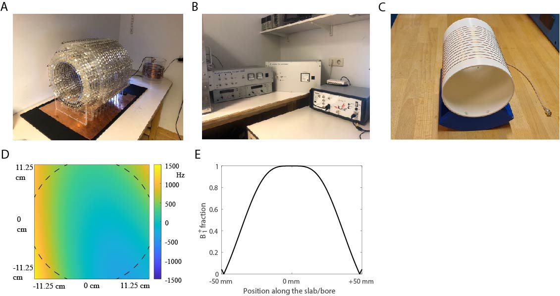
Figure 1. Experimental setup. (A) Halbach magnet. (B) Gradient amplifiers (left), RF amplifier (middle) and spectrometer (right). (C) solenoid transceive RF coil. (D) ΔB0 field in Hz with respect to the center frequency, measured with a robot. (E) RF excitation profile along the bore.
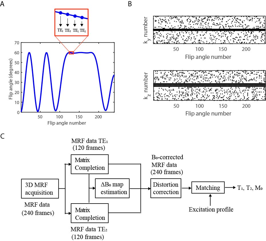
Figure 2. Fingerprinting sequence and reconstruction pipeline. (A) The MRF sequence uses a flip angle train of 240 RF shots and an alternating TE pattern similar to that in Ref. 8. (B) The 3D sampling pattern. The sampled phase encoding numbers are plotted for each of the RF shots. (C) The MRF data is reconstructed using matrix completion, after which a ΔB0 map is estimated from the TE difference. The ΔB0 map is used to correct for B0-induced image distortions in the MRF images, before matching the data to the dictionary.
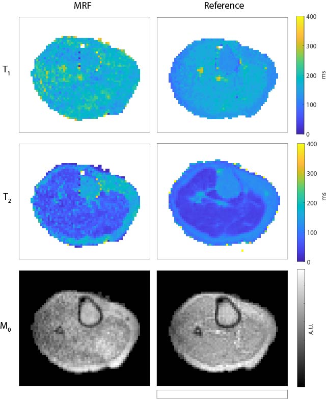
Figure 3. Comparison of relaxation time maps obtained with MRF and with reference techniques in the lower leg. The muscle T1 times measured with MRF are in the same range as those measured with an inversion recovery sequence (175 ms vs 165 ms), but the muscle T2 times measured with MRF are longer than those measured with MESE (60 ms vs 40 ms). The SNR of the MRF maps is lower, as expected. Scan parameters for inversion recovery: TE/TR = 12/900 ms, echotrain length (ETL) = 5. Scan parameters for multi-ech-spin-echo: TR = 1250 ms, echotrain length (ETL) = 5.
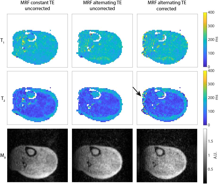
Figure 4. Comparison between uncorrected MRF data with constant TE and uncorrected and corrected MRF data with alternating TE. The relaxation time maps obtained from the MRF scan with an alternating TE pattern (without distortion correction) are very similar to those obtained with a constant TE pattern. A ΔB0 map was estimated from the alternating TE data and used to correct for image distortions along the readout direction before matching. The effects are small, but visible in the M0 maps and in the subcutaneous fat region in the T2 maps.
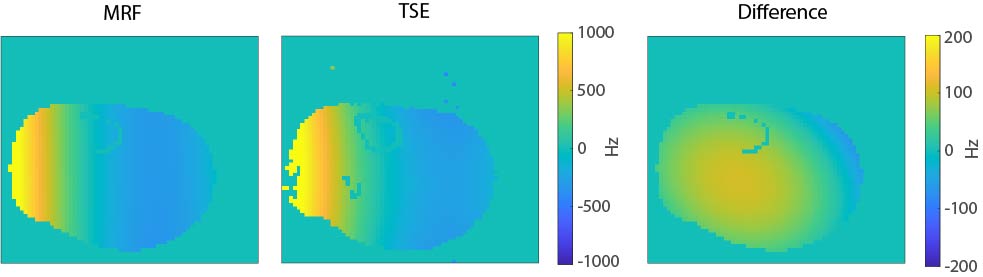
Figure 5. Comparison of the MRF-based ΔB0 map estimation with a standard TSE-based technique. The ΔB0 map estimated from the MRF data is close to that obtained with a TSE sequence. The maximal difference is 105 Hz, which could be caused by phase errors in the MRF sequence due to system imperfections or temperature induced B0 drift, which can be as much as 1500 Hz/hour during in-vivo imaging. Scan parameters for the TSE sequence: resolution = 2.5×2.2×3.0 mm3, TE/TR = 12/300 ms, readout gradient shift = 150 µs, echotrain length (ETL) = 5, scan time = 9 min.
DOI: https://doi.org/10.58530/2022/2516