2514
Joint sparsity multi-component MRF reconstruction - directly from k-space to component maps1Imaging Physics, Delft University of Technology, Delft, Netherlands, 2Department of Radiology, Leiden University Medical Centre, Leiden, Netherlands, 3Department of Radiology and Nuclear Medicine, Erasmus MC, Rotterdam, Netherlands
Synopsis
The use of high undersampling factors and short flip angle trains leads to shorter acquisition times in MR Fingerprinting acquisitions. To obtain accurate multi-component estimates from this data advanced reconstructions are required. We study a low-rank ADMM based reconstruction method that adds a multi-component constraint to the inverse reconstruction problem (MC-ADMM). This method is combined with a joint-sparsity constraint yielding higher quality multi-component estimates with k-SPIJN than with previous methods. In simulations we observed increased stability to sequence truncation and in vivo multi-component estimates contained less noise-like effects.
Introduction
MR Fingerprinting(MRF)1 allows for time-efficient estimation of tissue properties by sampling the MR-signal in a transient state while applying high undersampling factors. Conventionally, the data is first reconstructed to (SVD-compressed) time frame images, from which parameter estimates per voxel are obtained, e.g. T1,T2 and M0-maps.This voxel-wise estimation does not take multi-component effects such as myelin water or partial voluming into account. Recently we proposed the Sparsity Promoting Iterative Joint NNLS algorithm for MRF-data(SPIJN-MRF) to obtain multi-component T1,T2-estimates based on a joint-sparsity constraint2. The estimation of multi-component fraction maps is less robust to artifacts than single-component estimations and therefore requires data with less undersampling artifacts (and thus requiring long scan times).
In this work we aim to improve the image reconstruction to facilitate multi-component MRF while high undersampling factors are applied. Therefore we propose an Alternating Direction Method of Multipliers(ADMM) including multi-component constraints into the reconstruction problem. The proposed k-SPIJN method benefits from this extra regularization term that enables direct estimation of joint sparsity multi-component estimates from undersampled data.
Methods
Reconstruction MethodEssentially, multi-component effects in MRF can be modeled as a linearly weighted combination of (low rank(LR)3) dictionary items D(Dr, rank r). Given certain LR-images xr, the weights of the dictionary items can be obtained by solving a non-negative least squares problem:$$c=\operatorname{argmin}_{\hat{c}\in\mathbb{R}^{N_d\times N_n}_{\geq 0}} \left\lVert\,P_rD_r\hat{c}-x_r\right\rVert_2^2,\qquad\,(1)$$in which$$$\,c\in\mathbb{R}^{N_d\times\,N_n}_{\geq\,0}\,$$$are estimated magnetization weights per voxel and dictionary atom, and Pr represents spatial phase variations (as excluded from the real-valued $$$c$$$). $$$P\in\mathbf{C}^{N_n}$$$ is calculated based on a LR-solution, using r=1, through$$P=\frac{x_1}{\operatorname{abs}(x_1)},\qquad\,(2)$$with element-wise division, after which $$$P$$$ is mapped to r dimensions ($$$P_r$$$).
The inverse multi-component reconstruction problem can be written as:$$c=\operatorname{argmin}_{\hat{c}\in\mathbb{R}^{N_d\times\,N_n}_{\geq 0}} \left\lVert\,GU_rF_rSP_rD_r\hat{c}-k\right\rVert_2^2.\qquad\,(3)$$ Where k is (multi-coil) k-space data, G a (spiral) gridding-operator, Ur a SVD-based compressionoperator, Fr a Fourier-operator, S a coil-sensitivity-operator and r−underscript denotes operators ”broadcasted” to low-rank space.
Since this problem can not be solved directly in an efficient manner, we performed variable splitting as Ässlander et al.4 did for single-component MRF. Accordingly, we rewrote the MC-MRF reconstruction as an augmented Lagrangian minimization problem:$$x_r,c,\bar{u}=\operatorname{argmin}_{\hat{x}_r,u\in\mathbb{C}^{r\times\,N_n},\hat{c}\in\mathbb{R}^{N_d\times N_n}_{\geq 0}}\frac{1}{2}\left\lVert\,GU_rF_rS_r\hat{x}_r-k\right\rVert_2^2+$$$$\frac{\mu}{2}\left\lVert\,P_rD_r\hat{c}-\hat{x}_r+u\right\rVert_2^2-\frac{\mu}{2}\left\lVert\,u\right\rVert_2^2,\qquad\,(4)$$in which u is the scaled Lagrange multiplier and µ the coupling parameter balancing data consistency and constraint terms.
Subsequently, a multi-component ADMM (MC-ADMM, Fig.1-upper row) was used to solve (4), alternating between:$$x_r=\operatorname{argmin}_{\hat{x}_r\in\mathbb{C}^{r\times N_n}}\frac{1}{2}\left\lVert\,GU_rF_rS_r\hat{x}_r-k\right\rVert_2^2+\frac{\mu}{2}\left\lVert\,P_rD_r\hat{c}-\hat{x}_r+u\right\rVert_2^2,\qquad\,(5a)$$$$c=\operatorname{argmin}_{\hat{c}\in\mathbb{R}^{N_d\times\,N_n}_{\geq\,0}}\frac{\mu}{2}\left\lVert\,P_rD_r\hat{c}-\hat{x}_r+u\right\rVert_2^2,\qquad\,(5b)$$$$u=u+x_r-P_rD_rc,\qquad\,(5c)$$until convergence was reached. The LR-inversion problem of (5a) was solved with Conjugate Gradients. (5b) was solved using the NNLS algorithm5.
To reduce the number of possible solutions and regularize the multi-component problem, the Sparsity Promoting Iterative Joint NNLS (SPIJN)2 (Fig.1-middle row) algorithm was applied, applying a joint-sparsity constraint minimizing the number of tissue components, i.e. in a voxel as well as spatially, regularizing the number of non-zero component-maps ci. The sparsity term $$$N_c=\sum_{i=1}^N\left\lVert c_i\right\rVert_0$$$ was implemented by combining dictionary reweighting6 and $$$\ell_1$$$-regularization7 with SPIJN regularization parameter λ = 0.15.
The number of employed dictionary atoms is reduced by the joint-sparsity constraint. This facilitates that in an iterative scheme the actually used dictionary and component maps can be restricted to non-zero elements to improve problem conditioning. The resulting reconstruction scheme will be referred to as k-SPIJN(Fig.1-lower row).
Experiments
Experiments were performed with a gradient-spoiled SSFP-MRF acquisition8 with a flip angle train of length 400 (and truncated in numerical experiments) as proposed in [9] and using TR=15ms,TE=4ms. Dictionary signals were simulated using EPG’s10(T1=100ms-5.2s,T2=10ms-3s 5%-increments). A constant-density spiral with a undersampling factor 32 was used.
The Brainweb phantom11,incorporating partial voluming of white matter(WM), gray matter(GM) and CSF, was used in numerical simulations to verify the implemented methods and sensitivity to ADMM-parameters. Geometric mean T1 and T2-values were evaluated for error analysis.
In vivo brain scans were performed, after informed consent was obtained, on a 3.0 T Philips Ingenia (Best, The Netherlands) MRscanner with a 32-channel head coil (FOV=240×240mm2, in plane resolution 1×1mm2 and 5mm slice thickness). Acquisition with a single flip angle train and 5/32 repeats were performed (delay time 6s).
Both for numerical and in vivo experiments joint sparsity multi-component estimates were obtained by 1) LR-inversion and subsequently SPIJN 2) MC-ADMM and subsequently SPIJN and 3) k-SPIJN.
Results and Discussion
In numerical simulations the MC-ADMM showed a fast and stable convergence behavior for all 4 considered error measures(Fig.2), after which we fixated µ=2×10⁻³ in further experiments.When sequence lengths were truncated in simulations from 400 to 300 and 200 time-points, obtained estimations showed increasing errors and errors in WM and GM became dominant in LR-inversion estimates at N=200 (Fig.3). k-SPIJN showed lower errors than MC-ADMM estimates.
Estimated magnetization fraction maps with different reconstruction methods are shown in Fig.4 and Fig.5 for undersampling factors 5/32 and 1/32 respectively. All reconstructions yielded fraction maps corresponding to WM, GM and CSF. Also, myelin water fraction maps were estimated (shortest T1,T2 values, first column), but an increased noise propagation was observed in the MC-ADMM with subsequently SPIJN estimates compared to k-SPIJN.
For 5/32-undersampling 2 CSF-like components were estimated as observed before2,12, while 1/32-undersampling yielded 1 CSF component. This was not directly related to the used regularization parameter.
Conclusion
The k-SPIJN reconstruction method is able to obtain myelin water fraction maps from highly undersampled MRF-data, which was not possible with previous methods, with relatively short flip angle trains, reducing acquisition time.Acknowledgements
This research was partly funded by the Medical Delta consortium, a collaboration between the Delft University of Technology, Leiden University, Erasmus University Rotterdam, Leiden University Medical Center and Erasmus Medical Center.
The authors want to thank Peter Börnert for fruitful discussions and Peter Koken, Mariya Doneva and Thomas Amthor for providing the MRF patch.
References
(1) Ma, D.; Gulani, V.; Seiberlich, N.; Liu, K.; Sunshine, J. L.; Duerk, J. L.; Griswold, M. A. Nature 2013, 495, 187–192, DOI: 10.1038/nature11971.
(2) Nagtegaal, M. A.; Koken, P.; Amthor, T.; Doneva, M. Magnetic Resonance in Medicine 2020, 83, 521–534, DOI: 10.1002/mrm.27947.
(3) McGivney, D. F.; Pierre, E.; Ma, D.; Jiang, Y.; Saybasili, H.; Gulani, V.; Griswold, M. A. IEEE Transactions on Medical Imaging 2014, 33, 2311–2322, DOI: 10.1109/TMI.2014. 2337321.
(4) Assländer, J.; Cloos, M. A.; Knoll, F.; Sodickson, D. K.; Hennig, J.; Lattanzi, R. Magnetic Resonance in Medicine 2018, 79, 83–96, DOI: 10.1002/mrm.26639.
(5) Lawson, C. L.; Hanson, R. J., Solving least squares problems; SIAM: 1974.
(6) Tropp, J. A. Signal Processing 2006, 86, 589–602, DOI: 10.1016/j.sigpro.2005.05.031.
(7) Foucart, S.; Koslicki, D. IEEE Signal Processing Letters 2014, 21, 498–502, DOI: 10.1109/ LSP.2014.2307064.
(8) Jiang, Y.; Ma, D.; Seiberlich, N.; Gulani, V.; Griswold, M. A. Magnetic Resonance in Medicine 2015, 74, 1621–1631, DOI: 10.1002/mrm.25559.
(9) Sommer, K.; Amthor, T.; Koken, P.; Meineke, J.; Doneva, M. In Proc. Intl. Soc. Mag. Reson. Med. 25, ISMRM: Honolulu, USA, 2017; Vol. 25, p 1491.
(10) Hennig, J. Journal of Magnetic Resonance 1988, 78, 397–407, DOI: 10.1016/00222364(88)90128-X.
(11) Collins, D. L.; Zijdenbos, A. P.; Kollokian, V.; Sled, J. G.; Kabani, N. J.; Holmes, C. J.; Evans, A. C. IEEE Transactions on Medical Imaging 1998, 17, 463–468, DOI: 10.1109/ 42.712135.
(12) Nagtegaal, M. A.; Koken, P.; Amthor, T.; de Bresser, J.; Mädler, B.; Vos, F.; Doneva, M. NeuroImage 2020, 219, 117014, DOI: 10.1016/j.neuroimage.2020.117014.
Figures
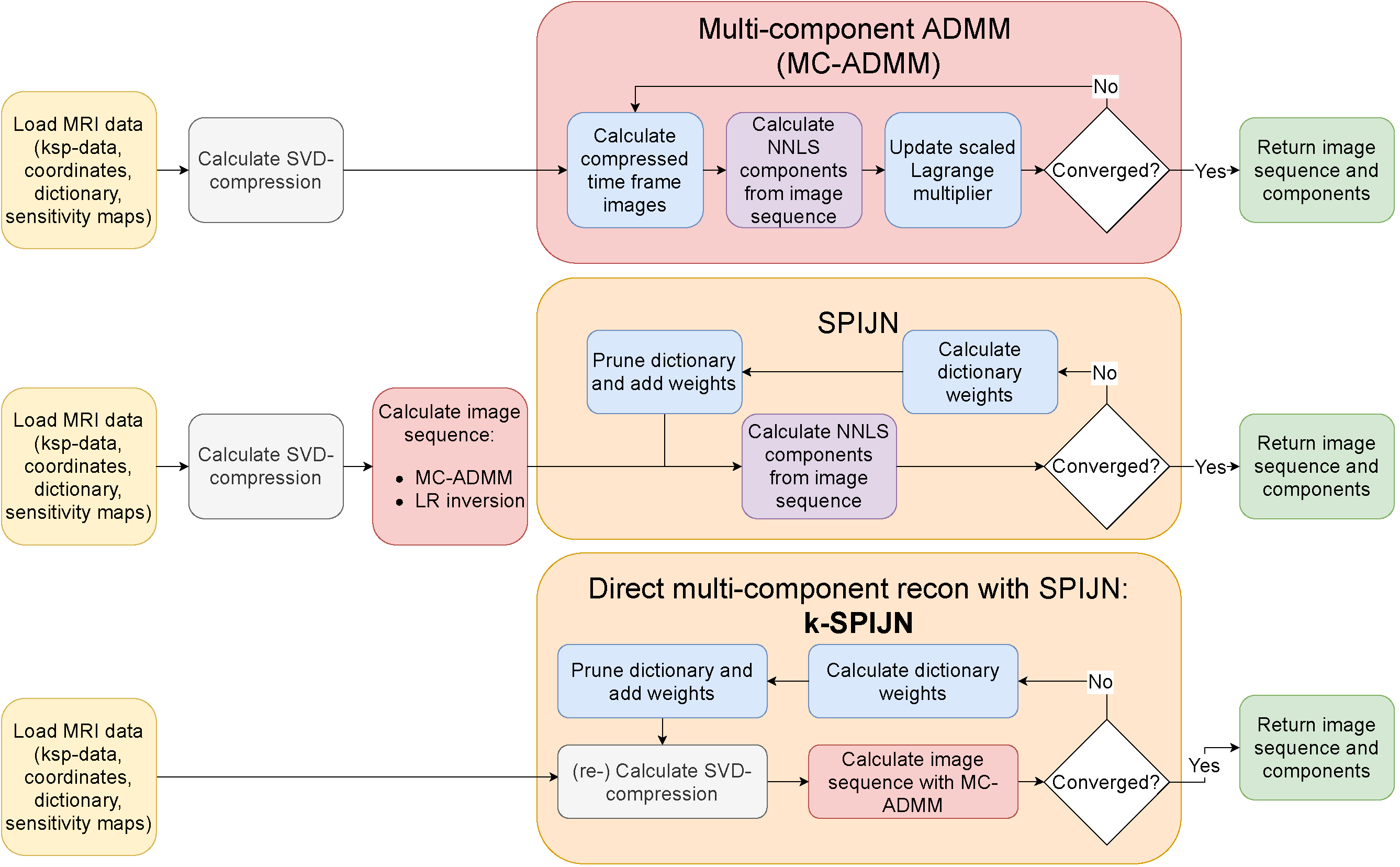
Figure 1: A schematic overview of the here proposed reconstruction methods. Low rank Multi-component ADMM (MC-ADMM) reconstructs low rank images with a multi-component constraint. SPIJN2 allows for joint-sparsity multi-component estimates from (low rank) images. k-SPIJN directly reconstructs joint-sparsity multi-component maps from undersampled k-space MRF data.
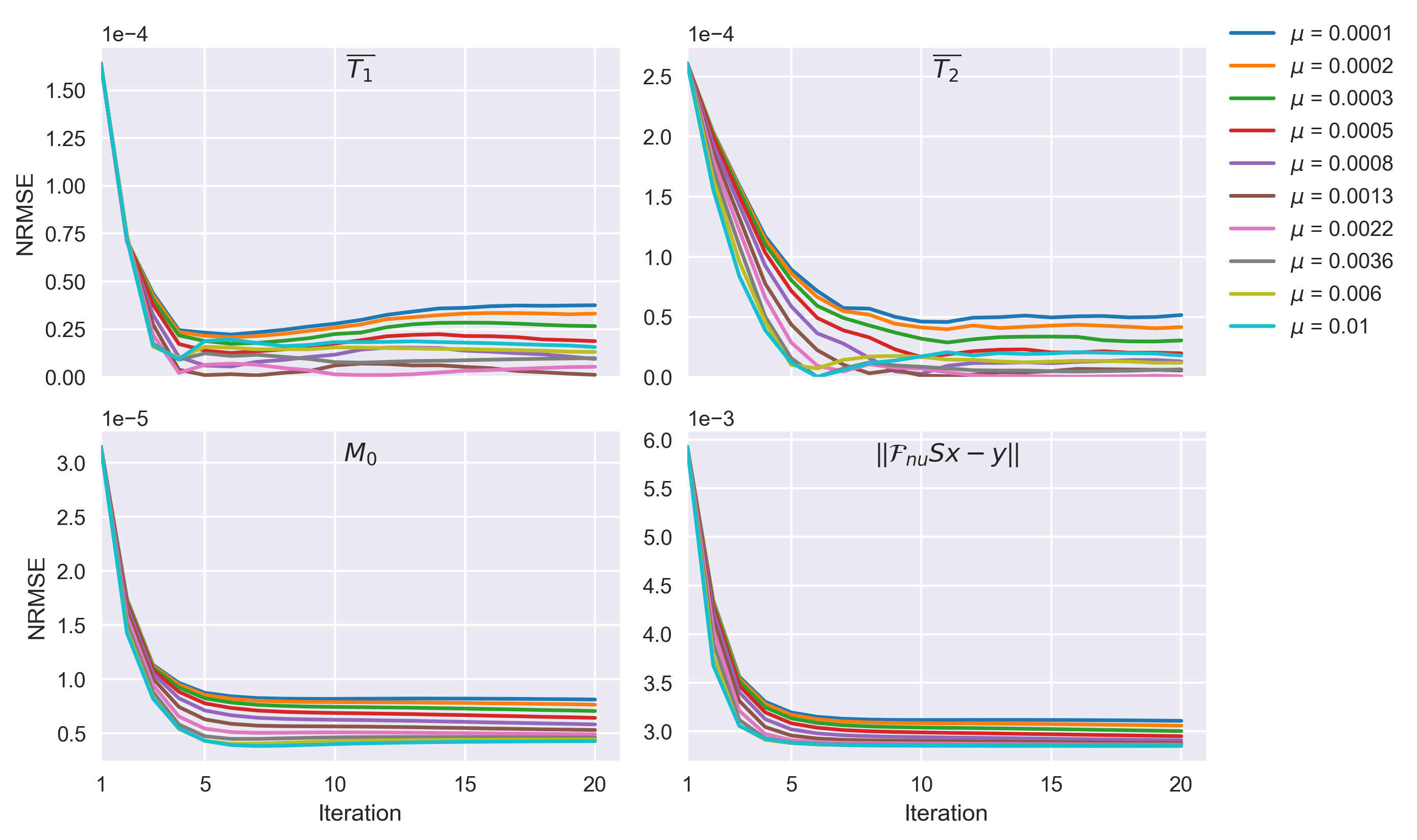
Figure 2: Convergence plots for different values of the ADMM coupling parameter. The ADMM loop was performed with 20 Conjugate gradient iterations per outer iteration. A numerical BrainWeb phantom was used as ground truth and the root mean square error (RMSE) is evaluated over the complete image. Geometric mean T1 and T2 were derived from the obtained component maps.
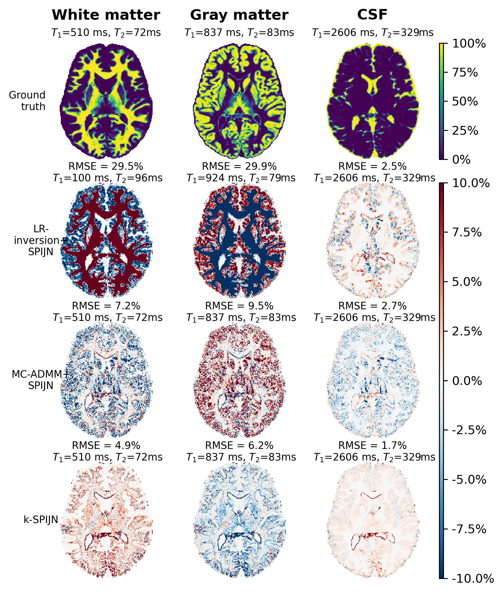
Figure 3: Obtained error maps for multi-component tissue segmentations using different reconstruction methods (lower 3 rows). A numerical BrainWeb phantom was used as ground truth (upper row) and an MRF sequence of length 200 was used. Root mean square errors (RMSE) were computed over the whole slice. Estimated and ground truth relaxation times are reported above each map.
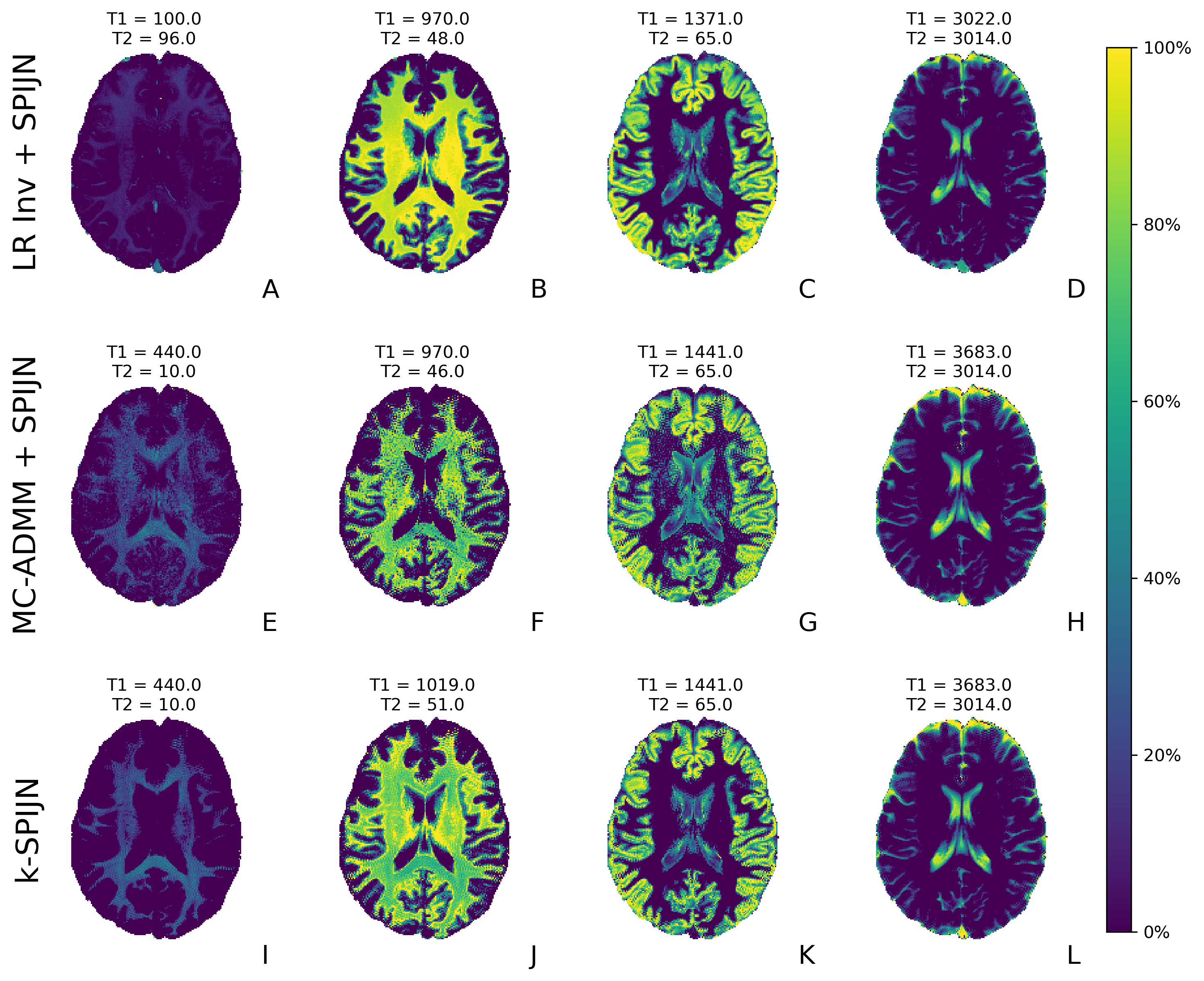
Figure 4: Estimated magnetization fraction maps and tissue components from R=5/32 undersampled data for sequence length 400 with 3 different reconstruction methods. The estimated components (structurally and matched relaxation times) relate to myelin water, WM, GM and CSF (columns from left to right). In general there is structural similarity between estimates, but k-SPIJN shows less noise especially in white matter. Remaining ringing artifacts can likely be removed by further tuning the regularization parameter and the tolerance level of CG.
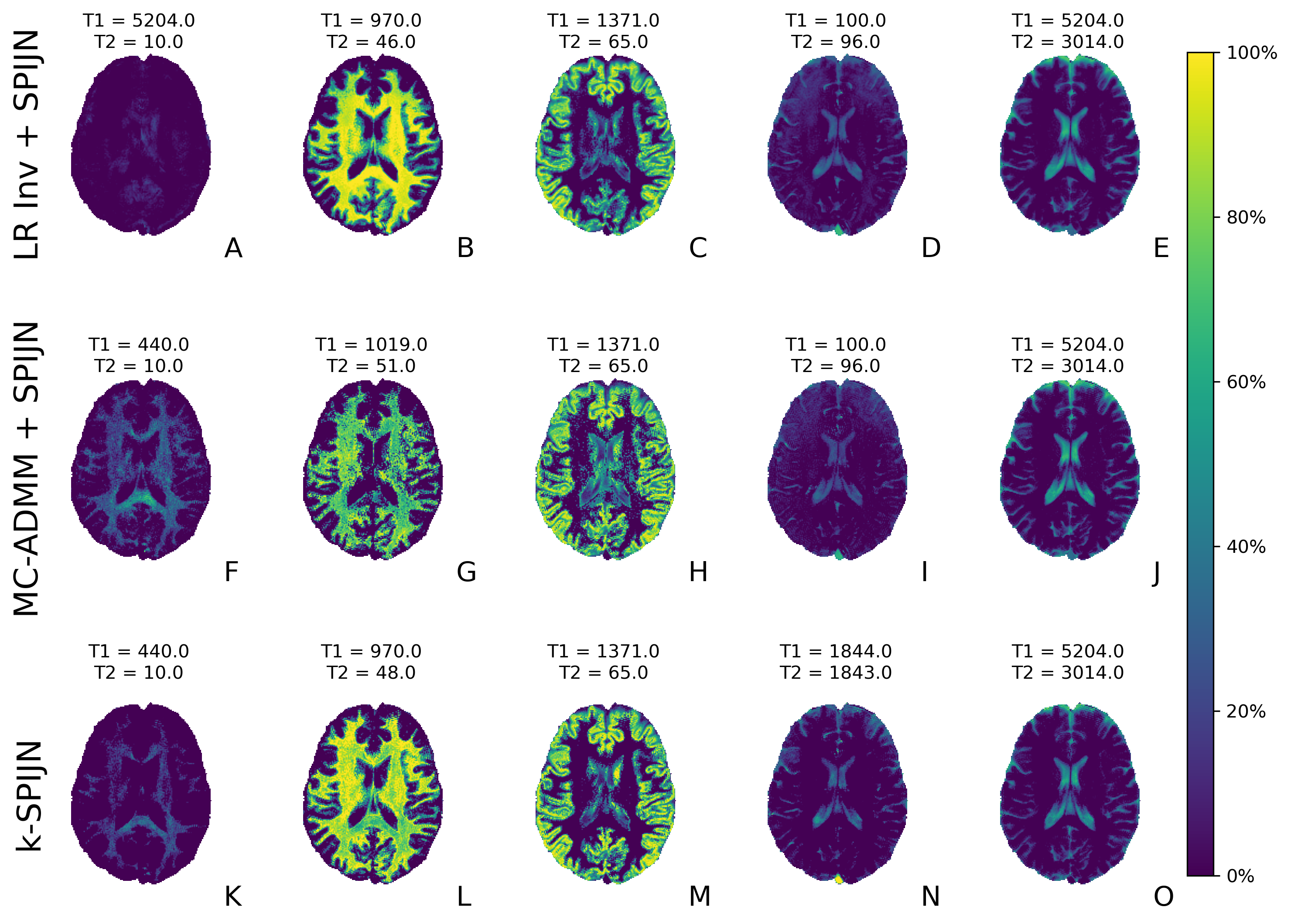
Figure 5: Estimated magnetization fraction maps and tissue components from R=1/32 undersampled data for sequence length 400 with 3 different reconstruction methods (rows). The estimated components (structurally and matched relaxation times) relate to myelin water, white matter, gray matter and CSF (2 components) (columns from left to right). Again differences between reconstruction techniques are most pronounced in the first 2 columns.