2491
Synthetic arterial spin labelling datasets of the kidneys for pipeline evaluation and comparison
Irène Brumer1, Dominik F. Bauer1, Lothar R. Schad1, and Frank G. Zöllner1
1Computer Assisted Clinicial Medicine, Mannheim Institute for Intelligent Systems in Medicine, Medical Faculty Mannheim, Heidelberg University, Mannheim, Germany
1Computer Assisted Clinicial Medicine, Mannheim Institute for Intelligent Systems in Medicine, Medical Faculty Mannheim, Heidelberg University, Mannheim, Germany
Synopsis
Synthetic kidney ASL data with respiratory motion was generated using models from the XCAT phantom and matching recommendations for in-vivo acquisitions. Both pCASL and PASL datasets with 1 M0 and 25 control-label pairs were created and analysed using an in-house developed processing pipeline including registration, manual segmentation, calculation of mean perfusion-weighted image and perfusion map. The registration performed well on the synthetic data and the perfusion maps yielded good cortex/medulla contrast. The presented method allows a wide range of parameter choices for creating synthetic ASL datasets valuable for testing processing pipelines and comparing them across research and clinical imaging centres.
Introduction
Perfusion imaging and quantification is important for diagnosing and monitoring numerous pathologies in different organs1-3. Compared to other modalities and techniques, arterial spin labelling (ASL) presents the advantage of being completely non-invasive1. However, the acquisition and processing of the data can be challenging, especially in the presence of motion. Because of these challenges, simulated data mimicking in-vivo acquisitions is of great value to test processing pipelines or even compare pipelines from different imaging centres. The aim of this project was to generate synthetic ASL datasets of the kidneys simulating in-vivo acquisitions for pipeline evaluation and comparison purposes.Methods
Starting from a model of the XCAT phantom4, MR images were generated using a spin echo sequence with TR=5000ms, TE=23ms, coronal-oblique slice positioning, and voxel dimension 3x3x5mm3. These settings were chosen to match recommendations for in-vivo acquisitions2. Literature values were used for tissue specific parameters (proton density, T1, T2) of organs in the abdomen for a field strength of 3T5-7. The field of view of the generated MR images was adapted to in-vivo ASL acquisitions and Rician noise was added to reproduce signal-to-noise ratio similar to in-vivo acquisitions. The respiratory motion during a free breathing acquisition was simulated by generating 100 MR images at equally spaced time points around the exhalation part of the breathing cycle. The generated proton-density weighted MR images with respiratory motion were used as basis for the M0 and multiple control-label pairs. Matching previous in-vivo acquisitions, we chose 25 control-label pairs, resulting in 51 images randomly selected from the available 100 time points. Background suppression used for control and label images was modelled by reducing the signal intensity of all control and label images to 20% of the signal of the M0 image (Figure 1). A perfusion ratio of 5 was assumed between cortex and medulla8. The general kinetic model9 was used to create both pseudo-continuous ASL (pCASL) and pulsed ASL (PASL) datasets, assuming arterial transit times of 1123ms and 1141ms for the medulla and cortex10, respectively. Single-slice synthetic ASL datasets were then analysed using our in-house developed processing pipeline running in MATLAB 2020a (The MathWorks, Inc., Natick, Massachusetts, USA). Rectangular masks were manually drawn on the M0 image to register left and right kidneys separately (Figure 2(a)). A multi-resolution groupwise parametric registration was used to register all 51 images of the dataset using the Elastix toolbox11,12. The quality of registration was evaluated by looking at line profiles across the time dimension of the ASL dataset as well as calculating mean structural similarity index measures (MSSIMs)13 for all possible image pairs of the dataset. The mean perfusion-weighted image was calculated by pair-wise subtraction of control and label images followed by averaging. The perfusion was quantified using the following equations:for pCASL data $$rbf \ [mL/100g/min] = \frac{6000 \cdot \lambda \cdot \Delta M \cdot e^{-PLD/T_{1b}}}{2 \cdot \alpha \cdot 0.93^2 \cdot M0 \cdot T_{1b} \cdot (1-e^{-\tau/T_{1b}})}$$
for PASL data $$rbf \ [mL/100g/min] = \frac{6000 \cdot \lambda \cdot \Delta M \cdot e^{-TI/T_{1b}}}{2 \cdot \alpha \cdot 0.93^2 \cdot M0 \cdot TI_1}$$
A blood relaxation time $$$T_{1b}$$$ of 1650ms, a blood-tissue partition coefficient $$$\lambda$$$ of 0.9mL/100g, a labelling efficiency $$$\alpha$$$ of 0.85 and 0.95 for pCASL and PASL, respectively, and two background suppression pulses after labelling were assumed2. For the pCASL dataset, the post-labelling delay $$$PLD$$$ was 1200ms and the labelling duration $$$\tau$$$ was 1600ms. For the PASL dataset, the inversion time $$$TI$$$ was 1800ms and the labelling duration $$$TI_1$$$ was 1200ms. Segmentation was performed manually on the registered M0 image (Figure 2(b)).
Results
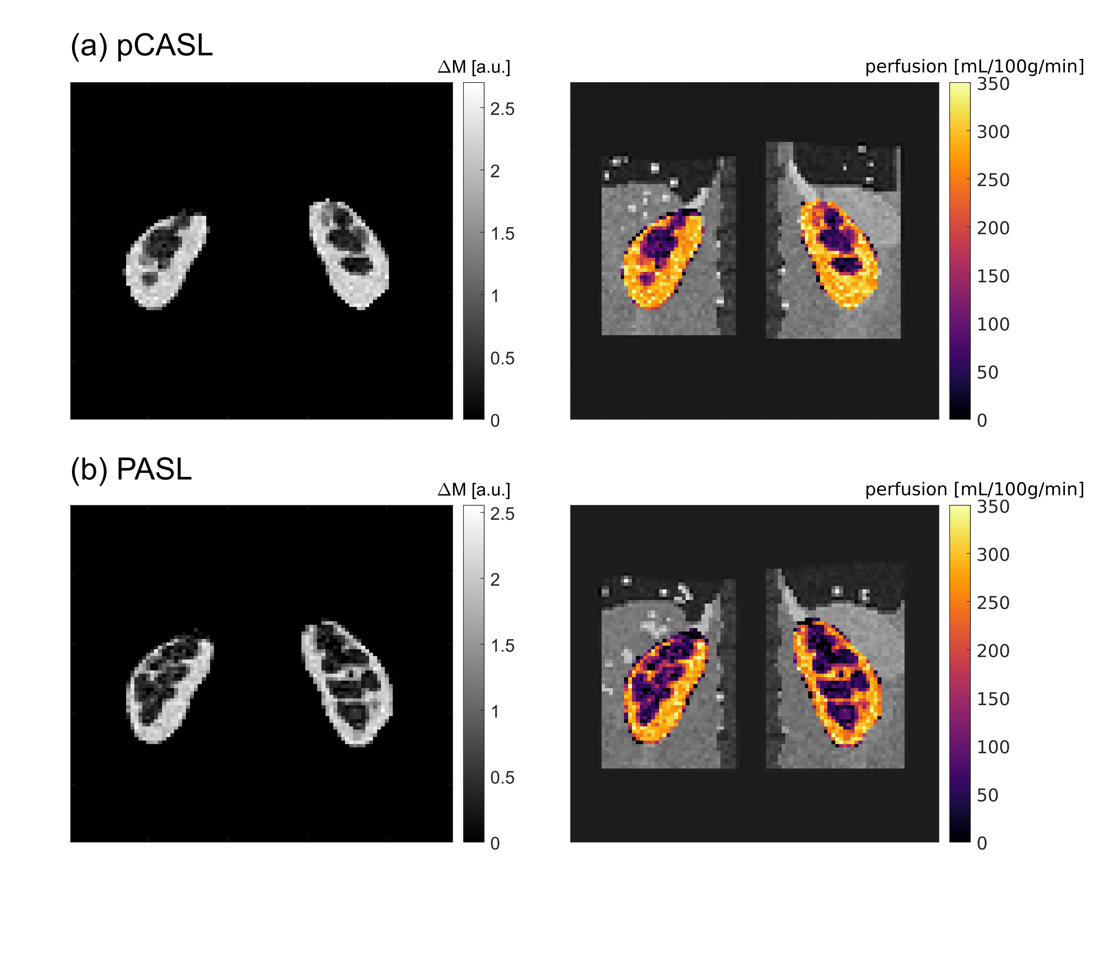
The M0, first label and first control images of a single-slice synthetic pCASL and PASL datasets are shown in Figure 1. The calculated perfusion-weighted image and the perfusion map for the same datasets are shown in Figure 3. Mean renal blood flow values were 218+/-51mL/100g/min and 209+/-48mL/100g/min for the left and right kidney respectively for the pCASL dataset and 166+/-49mL/100g/min and 167+/-49mL/100g/min for the left and right kidney respectively for the PASL dataset. Horizontal and vertical line profiles for both kidneys of the pCASL dataset are shown in Figure 4 and MSSIMs for each image pair of the pCASL dataset are shown in Figure 5. For the pCASL dataset, MSSIMs ranged between 0.05 and 1 before and between 0.42 and 1 after registration. For the PASL dataset, MSSIMs ranged between 0.05 and 1 before and between 0.39 and 1 after registration.Discussion
Synthetic ASL datasets of the kidneys simulating in-vivo acquisitions were successfully generated. The analysis performed with our in-house developed processing pipeline yielded good cortex/medulla contrast and the registration performed well on the synthetic dataset as indicated by higher MSSIMs calculated after registration. MSSIMs always were lowest for comparison of controls and labels with M0 as is to be expected because of the background suppression. Beyond the parameters chosen for this abstract, the described method can be used to create ASL datasets with different acquisition sequences, TR, TE, voxel dimension, noise level, number of control-label pairs, $$$PLD$$$/$$$TI$$$, $$$\tau$$$/$$$TI_1$$$, and level of breathing motion to further test limitations of processing pipelines.Conclusion
Synthetic ASL datasets of the kidneys mimicking in-vivo acquisitions have been created and used to test our in-house developed processing pipeline.Acknowledgements
This project was supported by the German Federal Ministry of Education and Research (BMBF) under the funding code 01KU2102, under the frame of ERA PerMed. This research project is part of the Research Campus M2OLIE and funded by the German Federal Ministry of Education and Research (BMBF) within the Framework "Forschungscampus: public-private partnership for Innovations" under the funding code 13GW0388A.References
1. Essig M, Nguyen TB, Shiroishi MS, et al. Perfusion MRI: the five most frequently asked clinical questions. Am J Roentgenol. 2013;201(3):W495-W510. 2. Nery F, Buchanan CE, Harteveld AA, et al. Consensus-based technical recommendations for clinical translation of renal ASL MRI. Magn Reson Mater Phy. 2020;33(1):141-161. 3. Andescavage N and Limperopoulos C. Emerging placental biomarkers of health and disease through advanced magnetic resonance imaging (MRI). Exp Neurol. 2020;347:113868. 4. Segars WP, Sturgeon G, Mendonca S, et al. 4D XCAT phantom for multimodality imaging research. Med phys. 2010;37(9):4902-4915. 5. Wissmann L, Santelli C, Segars WP et al. MRXCAT: Realistic numerical phantoms for cardiovascular magnetic resonance. J Cardio Magn Reons. 2014:16(1):1-11. 6. De Bazelaire CM, Duhamel GD, Rofsky NM et al. MR imaging relaxation times of abdominal and pelvic tissues measured in vivo at 3.0 T: preliminary results. Radiol. 2004;230(3):652-659. 7. Stanisz GJ, Odrobina EE, Pun J, et al. T1, T2 relaxation and magnetization transfer in tissue at 3T. Magn Reson Med. 2005;54(3):507-512. 8. Roberts DA, Detre JA, Bolinger L, et al. Renal perfusion in humans: MR imaging with spin tagging of arterial water. Radiol. 1995;196(1):281-286. 9. Buxton RB, Frank LR, Wong EC, et al. A general kinetic model for quantitative perfusion imaging with arterial spin labeling. Magn Reson Med. 1998;40(3);383-396. 10. Kim DW, Shim WH, Yoon SK, et al. Measurement of arterial transit time and renal blood flow using pseudocontinuous ASL MRI with multiple post‐labeling delays: Feasibility, reproducibility, and variation. J Magn Reson Imaging. 2017;46(3);813-819. 11. Klein S, Staring M, Murphy K, et al. Elastix: a toolbox for intensity-based medical image registration. IEEE. 2009;29(1):196-205. 12. Shamonin DP, Bron EE, Lelieveldt BP, et al. Fast parallel image registration on CPU and GPU for diagnostic classification of Alzheimer's disease. Front Neuroinform. 2014;7:50. 13. Wang Z, Bovik AC, Sheikh HR, et al. Image quality assessment: from error visibility to structural similarity. IEEE. 2004;13(4):600-612.Figures

Figure 1: Single-slice synthetic pCASL (a) and PASL (b)
datasets with M0, control 1 and label 1 images (left to right). The effect of
background suppression applied to control and label images for in-vivo acquisitions is
included in the synthetic dataset.
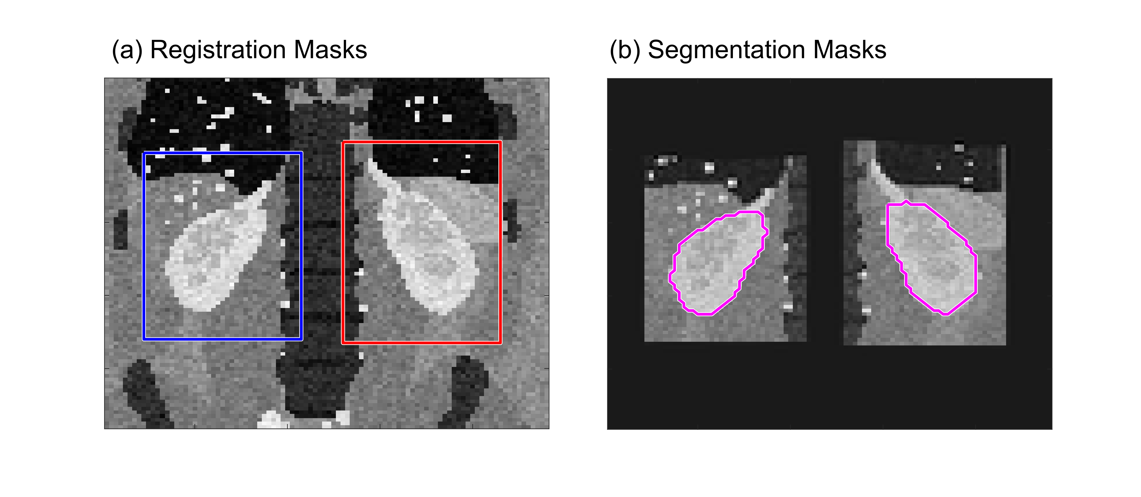
Figure
2: (a) Masks used for separate registration of left and right kidney overlaid
on the M0 image of the pCASL dataset. (b) Segmentation masks manually drawn on
the registered M0 image of the pCASL dataset.
Figure
3: Segmented mean perfusion-weighted image (left) and perfusion map overlaid on
registered M0 image (right) for the synthetic pCASL dataset (a) and the synthetic PASL
dataset (b).
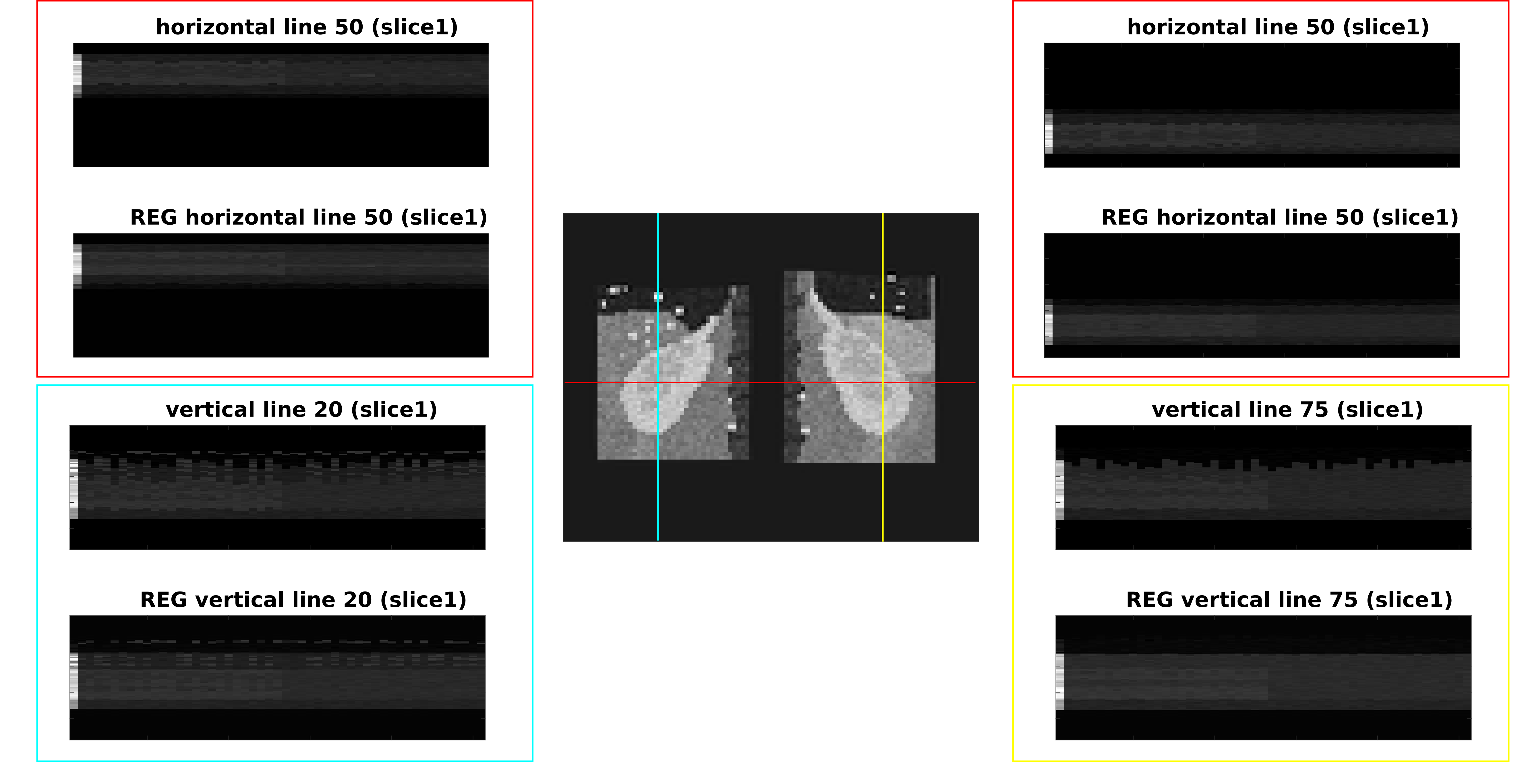
Figure
4: Horizontal and vertical line profiles of the left and right kidney of the
pCASL dataset before and after registration (REG). The chosen lines are displayed on
the registered M0 image in the centre. Along the vertical axis of the line profiles,
the images are ordered from left to right as 1 M0, 25 control, and 25 label images.
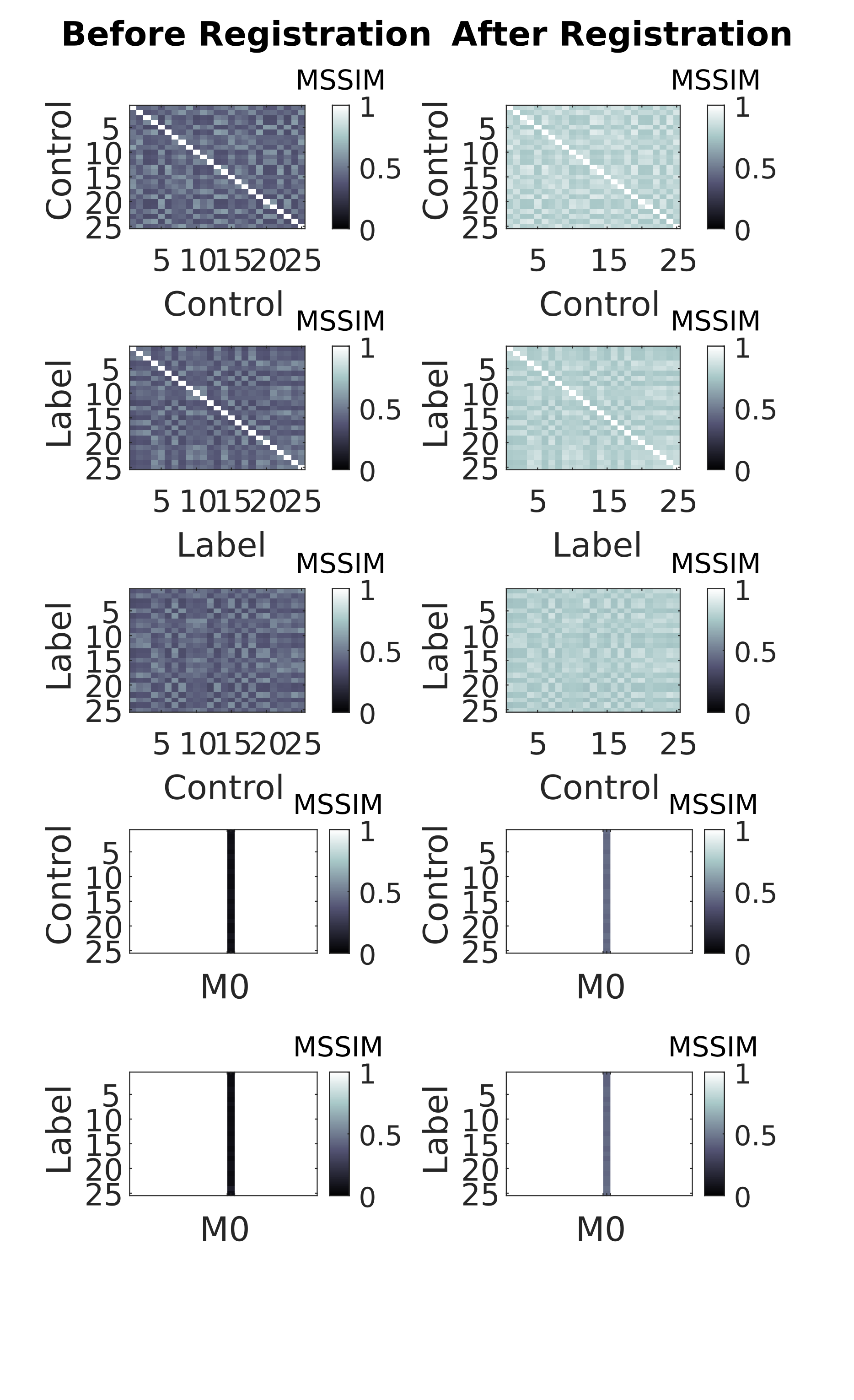
Figure
5: Mean structural similarity index measures (MSSIMs) calculated for each image pair
available in the pCASL dataset before registration (left) and after registration (right).
DOI: https://doi.org/10.58530/2022/2491