2467
A Proximal Step Enables Fast and Accurate Single-Step QSM Reconstructions, Preventing Susceptibility Underestimation1University College London, London, United Kingdom, 2Institute of Mathematics and Scientific Computing, University of Graz, Graz, Austria, 3Department of Neurology, Medical University of Graz, Graz, Austria, 4Department of Medical Physics and Biomedical Engineering, University College London, London, United Kingdom
Synopsis
Single-step quantitative susceptibility mapping (QSM) algorithms simplify the processing pipeline and promise to be more robust against background fields than traditional two-step methods but they often underestimate tissue susceptibilities. Here, we propose a highly efficient gradient descent Tikhonov-regularized proximal solver and a highly accurate ADMM TV-regularized proximal solver to improve the accuracy of two Laplacian-based single-step methods. Our solvers outperformed current single-step methods and showed in-vivo performance very similar to traditional two-step methods. This will simplify QSM processing pipelines, allowing further automation in future, although more research is needed to improve robustness against noise and boundary-conditions-related artifacts.
INTRODUCTION
Quantitative Susceptibility Mapping (QSM) solves an ill-posed inverse problem, where tissue susceptibilities are reconstructed from the phase of complex Gradient Echo acquisitions1. Traditionally, the QSM pipeline includes phase unwrapping and background field removal (BFR) steps. Previous research2 has shown that BFR methods leave residual background fields, mostly near boundaries of the region of interest (ROI), that create artifacts including streaking. Some BFR methods, may also remove local fields, yielding susceptibility underestimation. Aiming to alleviate these problems, several single-step QSM algorithms have been proposed3-8 that incorporate BFR into their formulation. Laplacian-based single-step algorithms are compatible with cutting-edge regularization strategies3,4, and could even incorporate phase unwrapping but they are prone to underestimation of susceptibility6. In this research we present two novel and highly efficient solvers for Laplacian-based single-step QSM and show that an additional proximal step prevents susceptibility underestimation.METHODS
Given that background fields are known to be harmonic inside the ROI, they have a zero-valued Laplacian. Hence, the Laplacian of the local field and the total field must be equal. This can be used explicitly in an optimization functional, similar to Chatnuntawech, et al.4 as follows:$$Laplacian-model:argmin_χ\frac{1}{2}\parallel m(\triangledown^2(d*χ)-\triangledown^2Φ)\parallel^2_2+Ω(χ)$$
where $$$m$$$ is the ROI binary mask, $$$\triangledown^2$$$ is the Laplacian operator, $$$d$$$ is the dipole kernel convolving the susceptibility distribution χ, Φ is the total field map and Ω(χ) is a suitable regularizer. Alternatively, it was proposed3 to introduce an auxiliary variable Ψ, where $$$\triangledown^2Ψ=\triangledown^2(d*χ)-\triangledown^2Φ$$$. Then, we solve the approximated equivalent model:
$$Graz-model:argmin_{χ,Ψ}\frac{1}{2}\parallelΨ\parallel^2_2 +\frac{σ}{2}\parallel m(\triangledown^2(d*χ)-\triangledown^2Φ-\triangledown^2Ψ)\parallel^2_2+Ω(χ)$$
Ψ is theorized to contain phase discrepancies, such as the background fields. Here σ is a penalty weight. In these two models, the Laplacian and dipole kernel convolution are merged into a single wave-like operator: $$$\frac{1}{3}\partial_x^2+\frac{1}{3}\partial_y^2-\frac{2}{3}\partial_z^2$$$.
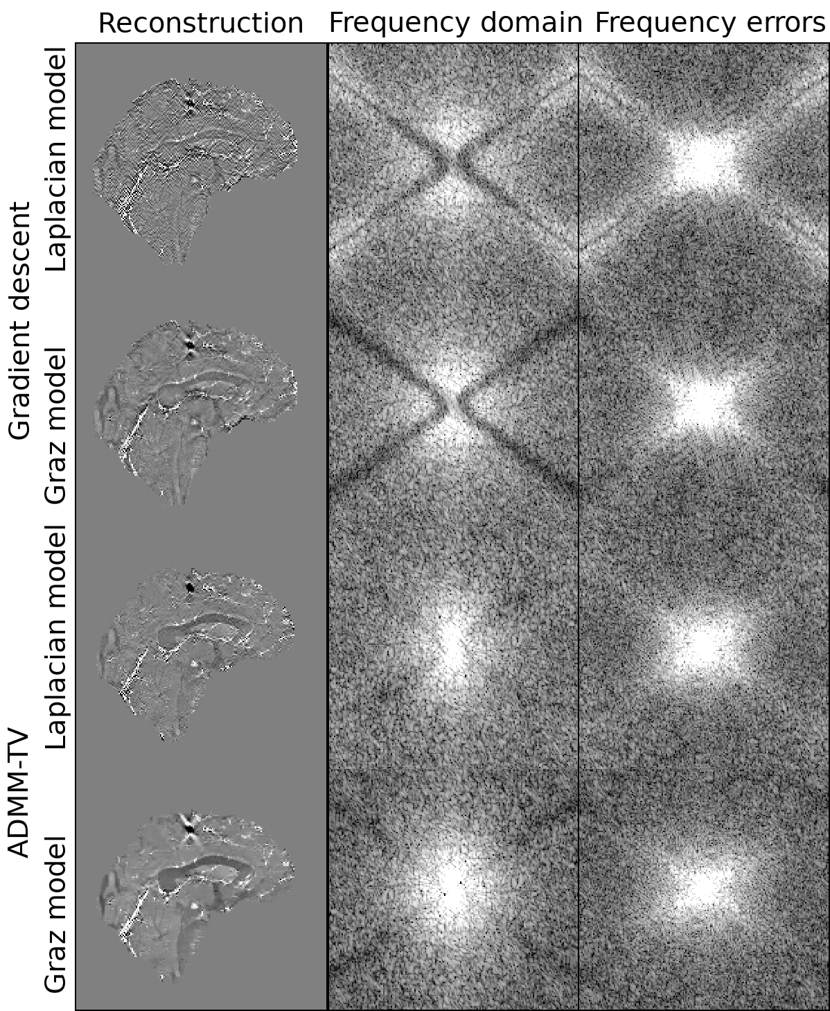
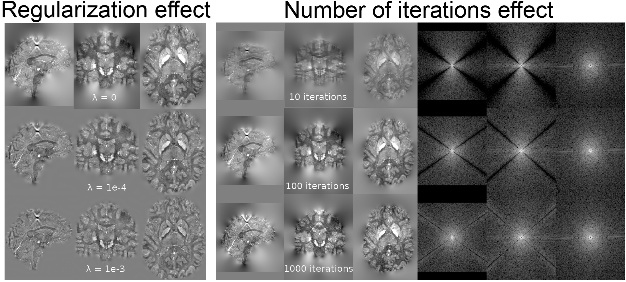
We propose two optimization solvers and corresponding regularizers for these two models. First, similarly to NDI9, we used a gradient descent solver and a Tikhonov regularization (GD-Tik), as this is a highly efficient algorithm that may be automated10. Second, similarly to FANSI11, we applied an ADMM solver with Total Variation regularization (ADMM-TV). Unfortunately, GD-Tik-based solvers are inefficient in recovering medium and low frequencies (Figure 1). Ψ also helps the Graz model to reduce noise, as shown by the attenuated high spatial frequencies near the cone at the magic angle. ADMM-based solvers are more efficient in recovering medium-scale features, but low frequencies are still mildly attenuated. For all these single-step solvers, we propose an additional proximal inner step, where $$$y=\triangledown^2χ$$$. This decouples the Laplacian and dipole kernels, which are used to update different variables. Whilst $$$y$$$ is updated using the dipole kernel by either the GD-Tik or the ADMM steps, χ is updated by the proximal operation. This proximal operation deconvolves the Laplacian operator (similar to a Wiener filter), recovering medium and low frequencies rapidly, and is only affected by the regularization weight. Figure 2 shows how the proximal Laplacian-model with GD-Tik solver is affected by different regularization weights and numbers of iterations.
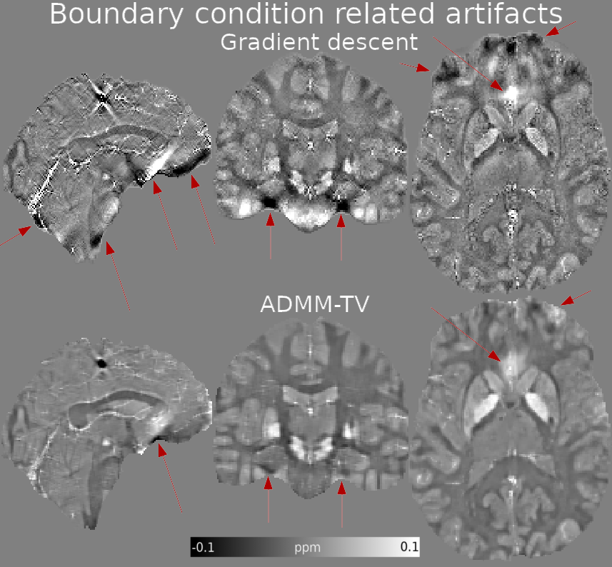
To minimize boundary-condition-related artifacts (as shown in Figure 3 for the proximal Graz-model solvers) in the proximal GD-Tik solvers we used a dynamic Tikhonov weight: $$$λ_n=2^{-n/5}$$$ where $$$n$$$ is the current iteration number. A 3-voxel ROI erosion was performed in all cases.
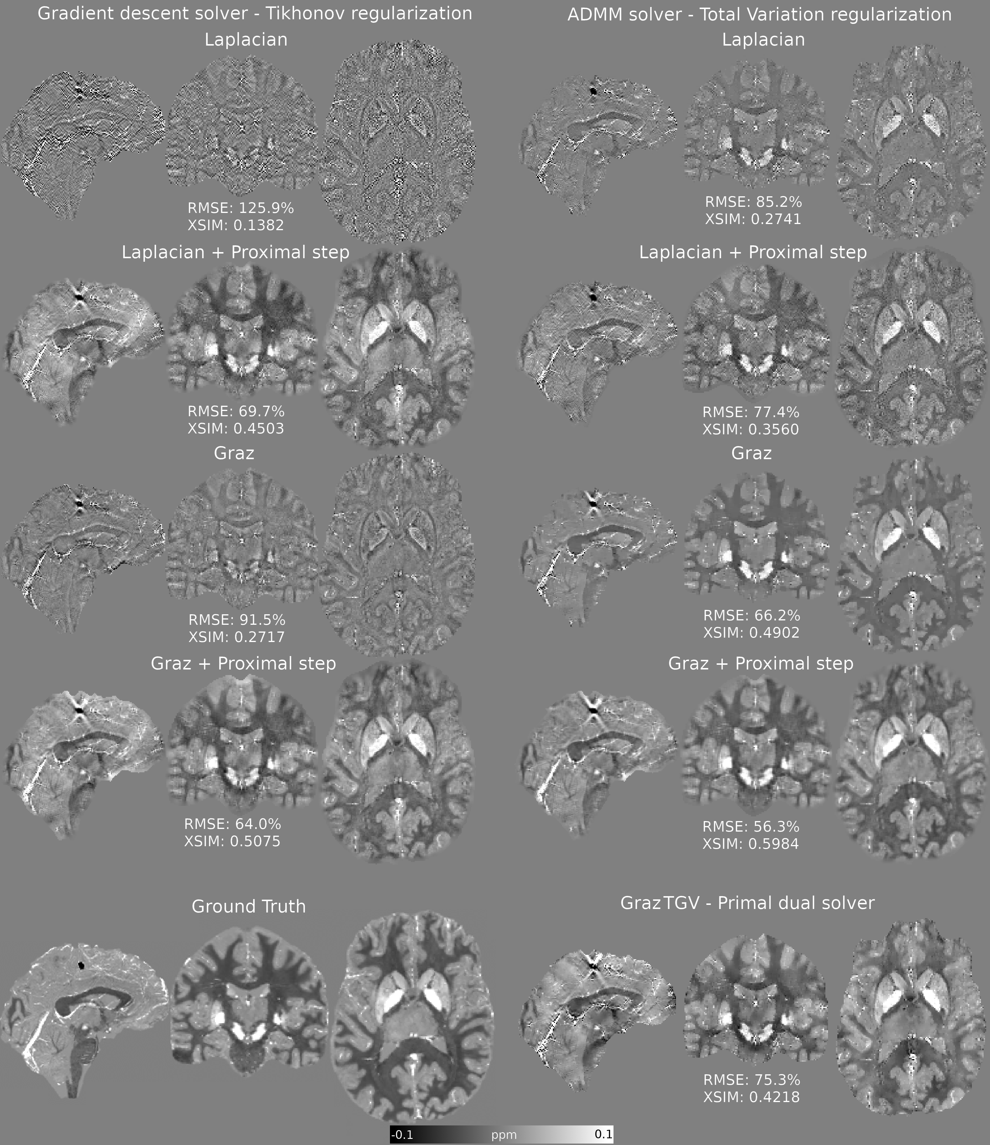
To assess the accuracy of these algorithms, we used a synthetic realistic total field simulation based on the 2019 QSM Reconstruction Challenge (RC2) phantom12 but with additional background fields. We added Gaussian noise to the simulated complex multi-echo Gradient Echo images and calculated the field map using a nonlinear complex fit13. We optimized the regularization weights and number of iterations to minimize RMSE and also calculated the XSIM14, and included the GrazTGV single-step method (primal-dual solver)3 for comparison. We compared reconstructions using these optimal regularization parameters in vivo on 3T (Achieva, Philips Healthcare, NL) acquisitions with a 32-channel head-coil and a 3D GRE sequence with 5 echoes, TE1/ΔTE/TR=3/5.4/29ms, flip angle=20°, matrix size = 240×240×144, and 1mm3 isotropic voxels15. For comparison, we performed two-step NDI (non-regularized, with automatic stopping10) and FANSI following BFR with PDF16.
RESULTS
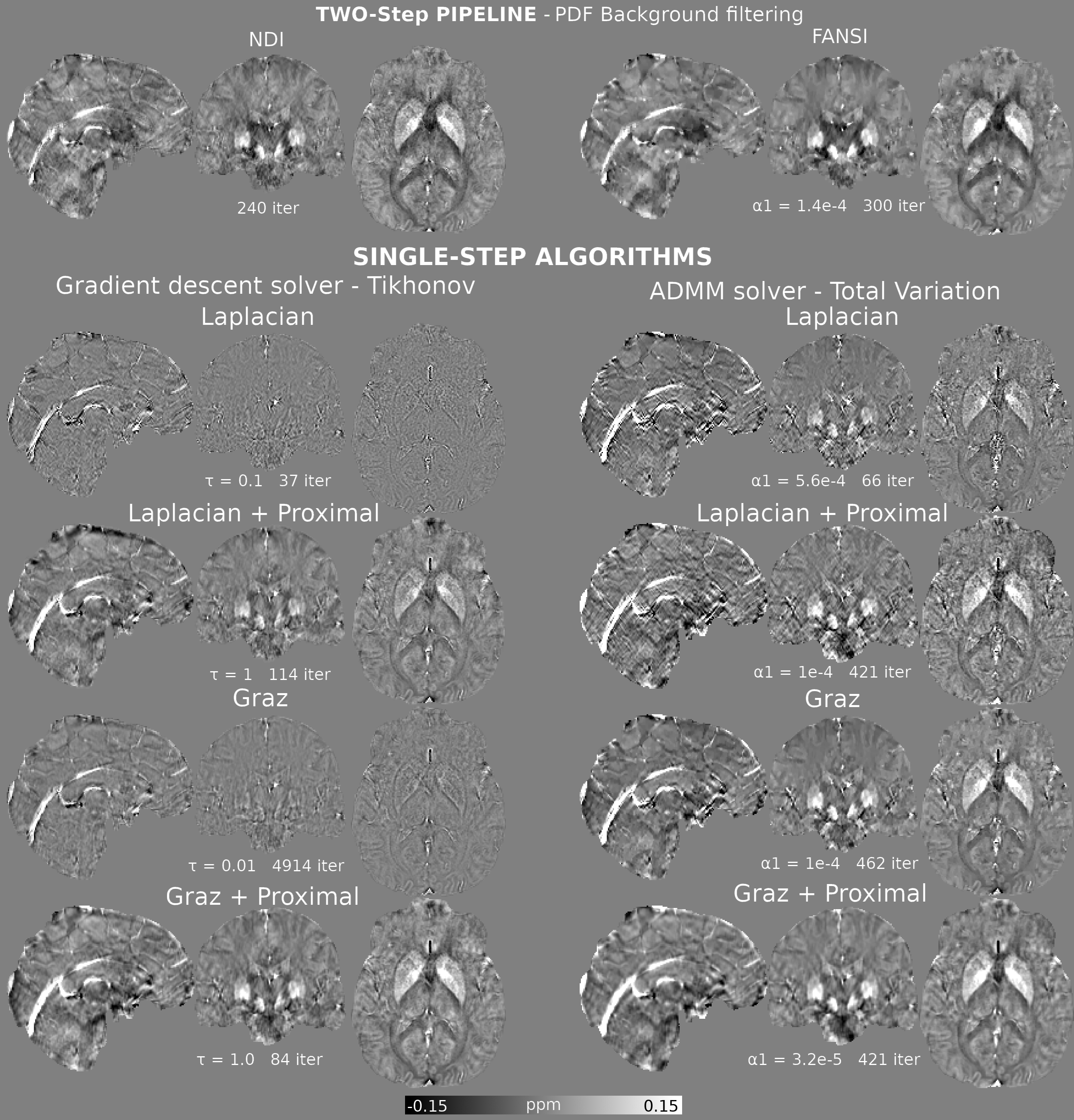
Optimal reconstructions for the simulated total field dataset are shown in Figure 4. The introduction of the proximal step increased the accuracy of all methods. The proximal Graz+ADMM-TV method achieved the best scores, although the GD-Tik solver was much more efficient (1092s for 421 iterations and 75s for 114 iterations, respectively). ADMM-TV regularized solutions were more robust against boundary condition artifacts than GD-Tik solutions (Figure 3). In-vivo reconstructions (Figure 5) achieved similar results to simulations, with Graz-model proximal solvers showing very similar results to their two-step counterparts (using PDF).DISCUSSION
The proximal step was very efficient in preventing tissue underestimation for all methods, outperforming state-of-the-art comparable methods. As these solvers are more sensitive to boundary-condition-related artifacts, they required additional mask erosion to prevent them. As these are linear algorithms working in the Laplacian domain, their denoising performance is suboptimal. Despite these limitations, which merit future investigation, Laplacian-based algorithms can incorporate phase unwrapping into their formulation, allowing for further QSM pipeline automation.CONCLUSION
A simple proximal step improved the quality of Laplacian-based single-step QSM algorithms which provide a competitive alternative to cutting-edge two-step QSM pipelines. Further research is needed to improve noise management and artifact prevention.Acknowledgements
We thank Cancer Research UK Multidisciplinary Award C53545/A24348 for its funding support. Karin Shmueli is supported by European Research Council Consolidator Grant DiSCo MRI SFN 770939References
1. Shmueli K. Chapter 31 - Quantitative Susceptibility Mapping. Advances in Magnetic Resonance Technology and Applications, Academic Press, 2020(1):819-838. doi:10.1016/B978-0-12-817057-1.00033-0
2. Schweser, F., Robinson, S. D., de Rochefort, L., Li, W., and Bredies, K. (2017) An illustrated comparison of processing methods for phase MRI and QSM: removal of background field contributions from sources outside the region of interest. NMR Biomed., 30: e3604. doi: 10.1002/nbm.3604.
3. Langkammer C, Bredies K, Poser B, Barth M, Reishofer G, Fan AP, Bilgic B, Fazekas F, Mainero C, Ropele S. Fast quantitative susceptibility mapping using 3D EPI and total generalized variation. Neuroimage 2015;111:622-630.
4. Chatnuntawech I, McDaniel P, Cauley SF, Gagoski BA, Langkammer C, Martin A, Grant PE, Wald LL, Setsompop K, Adalsteinsson E, Bilgic B. Single-step quantitative susceptibility mapping with variational penalties. NMR Biomed. 2017;30:e3570. doi:10.1002/nbm.3570
5. Liu T, Zhou D, Spincemaille P, Yi W. Differential approach to quantitative susceptibility mapping without background field removal. In: Proceedings of the 22nd Annual Meeting of ISMRM, Milan, Italy. ; 2014:p597.
6. Liu Z, Kee Y, Zhou D, Wang Y, Spincemaille P. Preconditioned total field inversion (TFI) method for quantitative susceptibility mapping. Magn Reson Med. 2017;78:303-315. doi:10.1002/mrm.26331
7. Sun H, Ma Y, MacDonald ME, Pike GB. Whole head quantitative susceptibility mapping using a least-norm direct dipole inversion method. Neuroimage. 2018;179:166-175. doi: 10.1016/j.neuroimage.2018.06.036.
8. Milovic C, Bilgic B, Zhao B, Langkammer C, Tejos C, Acosta-Cabronero J. Weak-harmonic regularization for quantitative susceptibility mapping. Magn Reson Med. 2019;81:1399-1411.
9. Polak, D, Chatnuntawech, I, Yoon, J, et al. Nonlinear dipole inversion (NDI) enables robust quantitative susceptibility mapping (QSM). NMR Biomed. 2020;e4271. doi:10.1002/nbm.4271
10. Milovic C and Shmueli K. Automatic, Non-Regularized Nonlinear Dipole Inversion for Fast and Robust Quantitative Susceptibility Mapping. 29th International Conference of the ISMRM, 2021:p3982.
11. Milovic C, Bilgic B, Zhao B, Acosta-Cabronero J, Tejos C. Fast nonlinear susceptibility inversion with variational regularization. Magn Reson Med. 2018;80:814-821. doi:10.1002/mrm.27073
12. Marques JP, Meineke J, Milovic C, Bilgic B, Chan K-S, Hedouin R, van der Zwaag W, Langkammer C, and Schweser F. QSM Reconstruction Challenge 2.0: A Realistic in silico Head Phantom for MRI data simulation and evaluation of susceptibility mapping procedures. Magn Reson Med. 2021;86: 526– 542 doi:10.1002/mrm.28716
13. Liu T, Wisnieff C, Lou M, Chen W, Spincemaille P, Wang Y. Nonlinear formulation of the magnetic field to source relationship for robust quantitative susceptibility mapping. Magn Reson Med. 2013;69:467-476. doi:10.1002/mrm.24272
14. Milovic C, Tejos C, and Irarrazaval P. Structural Similarity Index Metric setup for QSM applications (XSIM). 5th International Workshop on MRI Phase Contrast & Quantitative Susceptibility Mapping, Seoul, Korea, 2019.
15. Karsa A, Punwani S, and Shmueli K. The effect of low resolution and coverage on the accuracy of susceptibility mapping. Magn Reson Med. 2019; 81: 1833– 1848
16. Liu T, Khalidov I, de Rochefort L, Spincemaille P, Liu J, Tsiouris AJ, Wang Y. A novel background field removal method for MRI using projection onto dipole fields (PDF). NMR Biomed. 2011;24:1129-36.
Figures