2463
A Comparison of Background Field Removal and “Single-Step” Algorithms in Realistic Phantoms: Towards QSM Challenge 3.0?1Department of Medical Physics and Biomedical Engineering, University College London, London, United Kingdom, 2Department of Neurology, Medical University of Graz, Graz, Austria, 3Donders Centre for Cognitive Neuroimaging, Radboud University, Nijmegen, Netherlands
Synopsis
The 2019 QSM Reconstruction Challenge compared how different algorithms reconstructed QSM from true local field maps. However, this neglects the importance of residual background fields, and how they degrade the solutions. Here, we used a realistic “total field” simulation to compare three different background field removal methods, and to estimate the susceptibility maps resulting from three state-of-the-art QSM algorithms. We also compared the performance of two single-step algorithms, that use the total field map as an input. Our results showed that the two-step Weak-Harmonic QSM method is robust against residual fields and achieved the lowest error scores, outperforming single-step methods.
INTRODUCTION
Quantitative Susceptibility Mapping (QSM) is increasingly used to study iron accumulation, calcifications, and demyelination in the brain1,2. QSM solves an ill-posed inverse problem, called dipole inversion, where susceptibilities are derived from the (“local”) magnetization fields generated by the objects in the region of interest (ROI)3. This process is prone to artifacts and is affected by pre-processing steps including phase unwrapping and background field removal (BFR). Therefore, numerous QSM algorithms have been proposed and were compared in the 2019 QSM Challenge (RC2)4. RC2 used realistic simulated noisy local field maps5 to quantify the accuracy of a wide range of dipole inversion algorithms. Background fields were not included in the simulated field maps and, therefore, robustness against residual background fields was not assessed. Here, we present a pilot study using the simulated SIM2 phantom created for RC2 with additional background fields. In contrast to a simple brain model used in a previous comprehensive comparison of BFR algorithms6 (which did not estimate their impact on QSM reconstructions), this SIM2 model includes a more realistic simulation of sources outside the ROI, including bone, tissue, and air cavities. We compared three popular BFR algorithms and evaluated their performance when combined with three cutting-edge dipole inversion algorithms. As BFR is implicitly included in “single-step” QSM algorithms7,8, we also compared the performance of two single-step algorithms, which use the total field as the input.METHODS
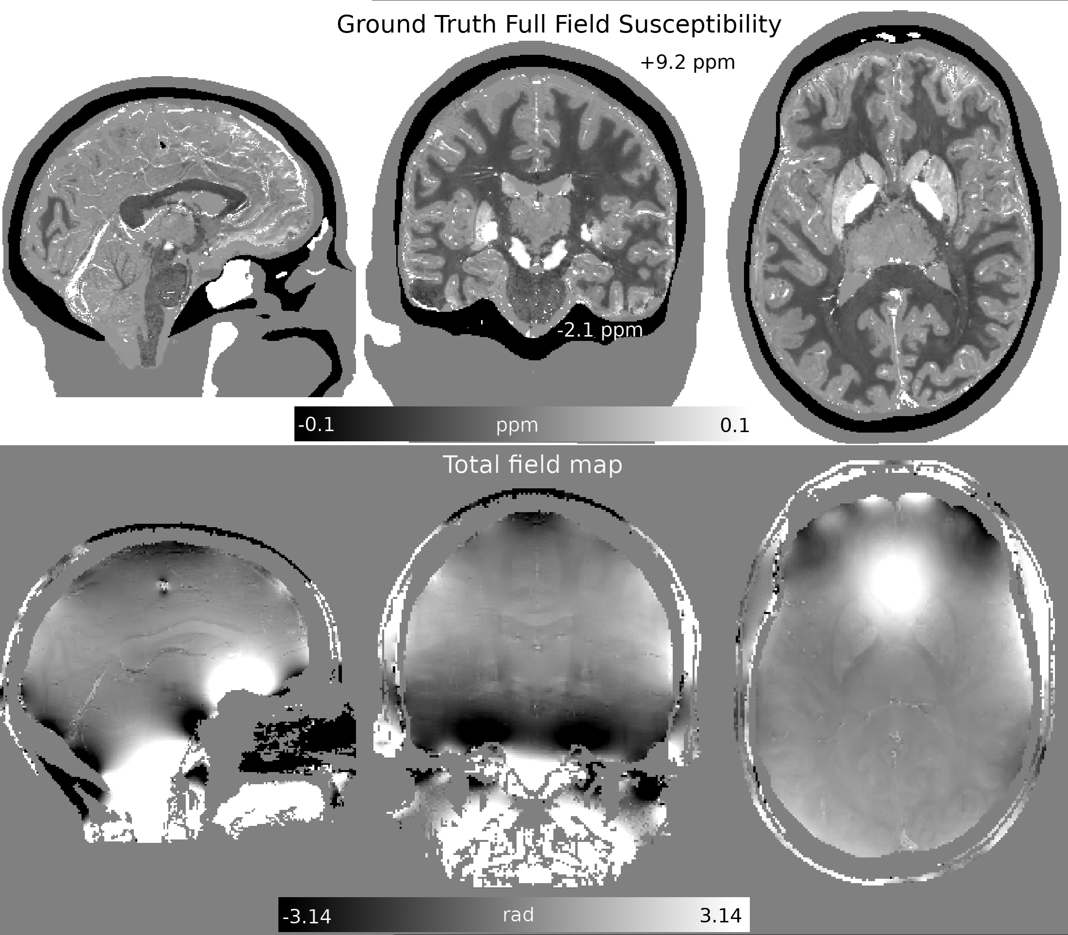
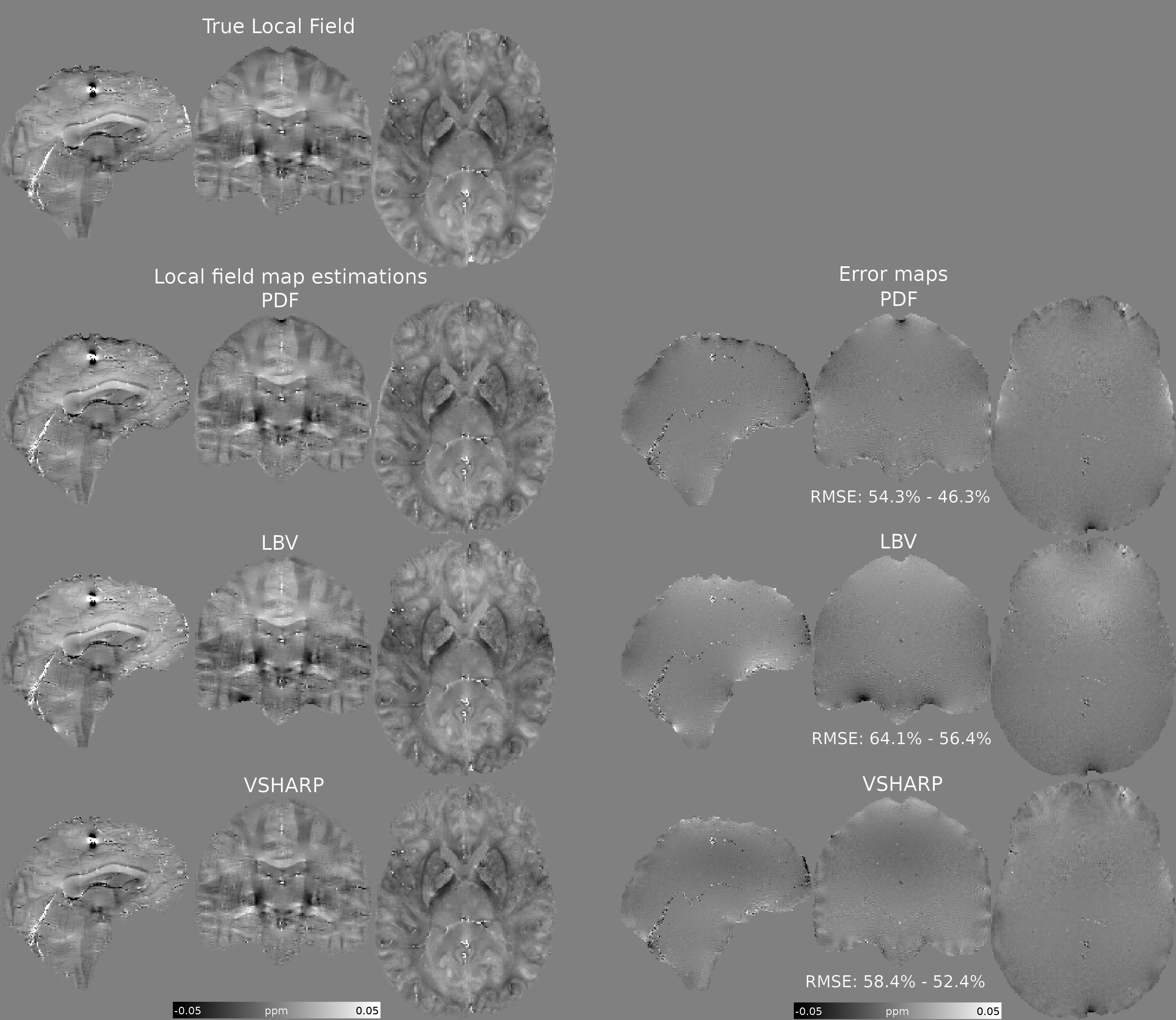
The toolbox used to simulate the ground truth and multi-echo acquisitions for RC25 includes a noiseless simulation (SIM2, which also included a strong calcification) with additional realistic background fields. We added noise (SNR=100) to the 1mm3 complex signals at all four TEs and performed a nonlinear multi-echo fit9 to estimate the total field map. To obtain the “true” local field map, we repeated this procedure on the (SNR=100) multi-echo simulation used in RC2 that did not include any background fields. Using the total field map (Figure 1) and the “true” local field map (Figure 2), we performed the following reconstructions and comparisons:1. BFR comparison. The Projection onto Dipole Fields Method (PDF)10, Laplacian Boundary Valued (LBV)11, and Variable Sophisticated Harmonic Artifact Reduction for Phase data (VSHARP)12 methods were applied to the total field map, using the supplied brain mask. Results were compared in terms of the Root-Mean-Squared-Error (RMSE) against the “true” local field map.
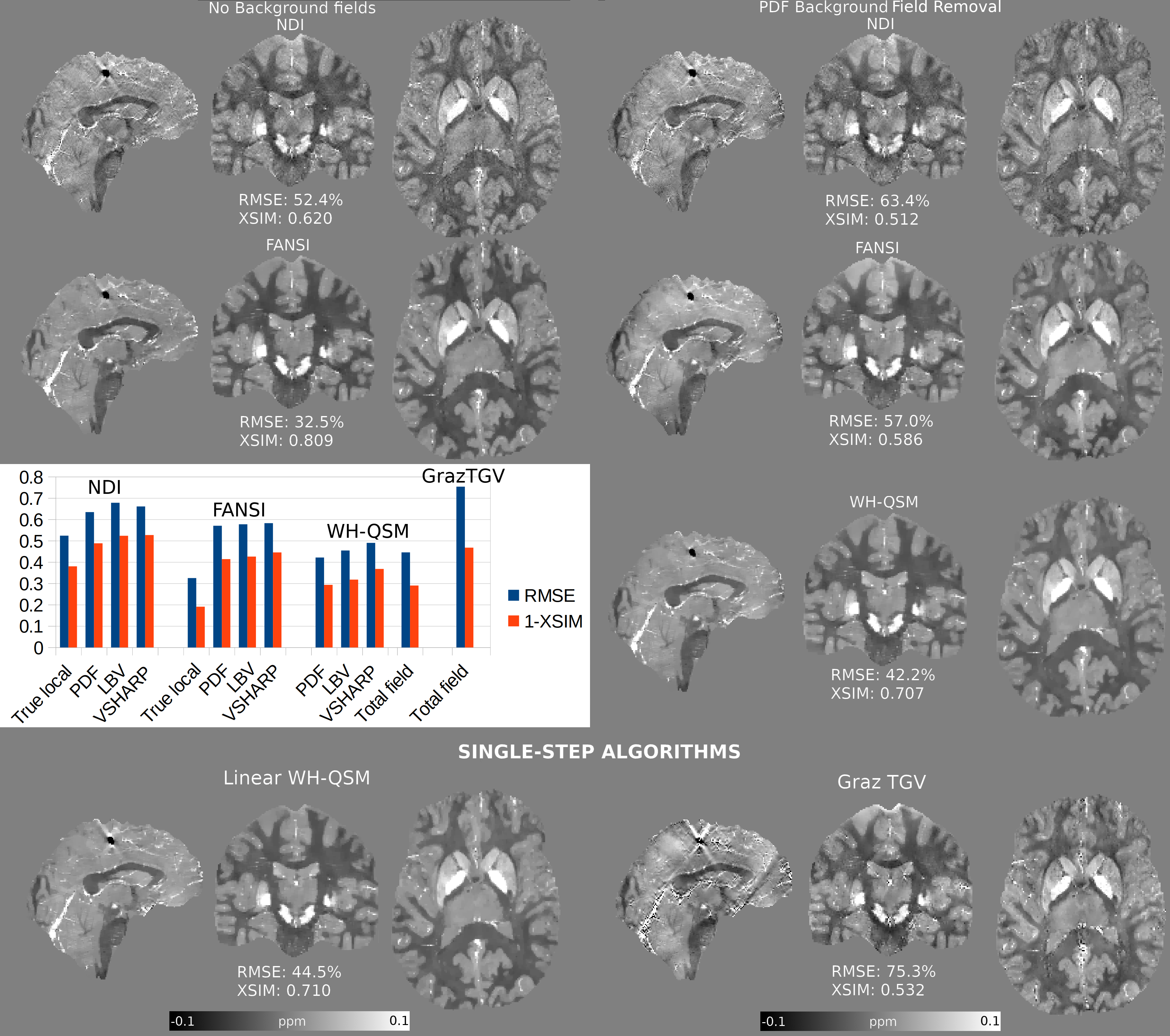
2. “Gold standard” QSM reconstructions were generated from the “true” local field map. We used Fast Nonlinear Susceptibility Inversion (FANSI13, winner of the RMSE category RC2, Stage 2) and Nonlinear Dipole Inversion (NDI14, a fast, non-regularized solver, reported to be robust against residual background fields) algorithms.
3. QSM reconstructions on the local field maps from 1.: We applied FANSI, NDI, and Weak Harmonic QSM (WH-QSM15, an extension to FANSI that incorporates joint estimation of residual background fields and dipole inversion).
4. Single-step reconstructions: We used the linear WH-QSM model with the total field as the input, without initialization or preconditioning. In addition, we used the GrazTGV single-step toolbox8. This algorithm inverts a wave-like operator instead of the dipole kernel and uses the Laplacian of the total field as the input. To prevent boundary-condition-related artifacts, the ROI mask (evaluation mask) was eroded by 3 voxels.
QSM reconstructions were optimized to minimize RMSE inside the RC2 evaluation mask. We also compared the Susceptibility-optimized Similarity Index Metric (XSIM)16 for all optimized reconstructions.
RESULTS
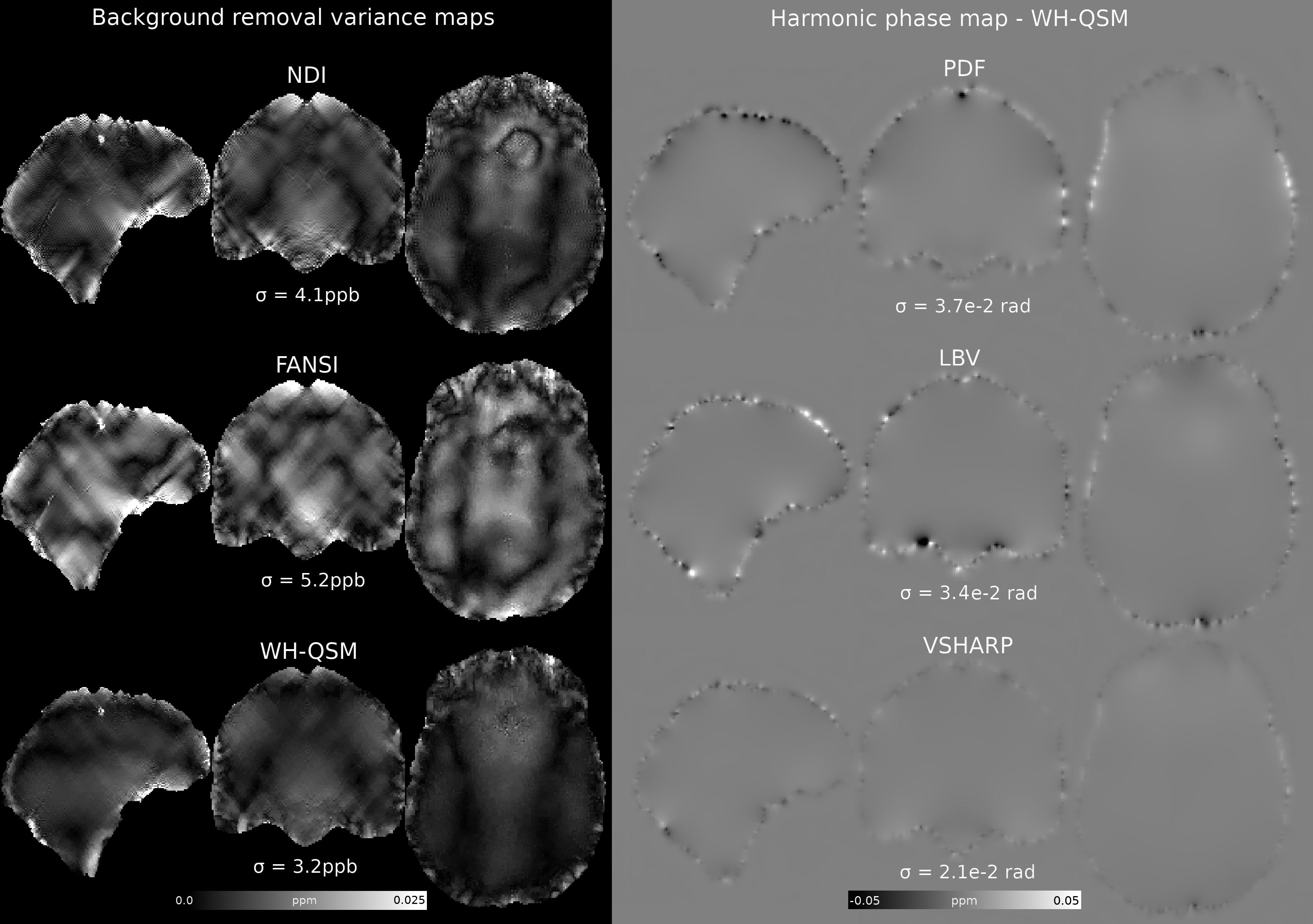
BFR results are shown in Figure 2, with PDF achieving the lowest errors in both the brain and evaluation masks. Gold-standard reconstructions, two-step, and single-step results are shown in Figure 3 (only optimal reconstructions using PDF BFR are shown). Two-step WH-QSM achieved the lowest RMSE and largest XSIM, for all methods, followed closely by the single-step WH-QSM. Two-step WH-QSM also showed the least variance across different local field inputs (more consistent results), and the harmonic phase residual estimates that it removes closely resemble the BFR error maps near the boundaries (Figure 4), demonstrating its efficiency in removing residual background fields.DISCUSSION
While VSHARP achieved lower errors than LBV in estimating the local field map, VSHARP’s error map reveals structural errors not present in other methods. VSHARP may suppress real local fields, and therefore result in worse QSM reconstructions. This is also suggested by WH-QSM’s harmonic phase estimation, which shows lower amplitude residuals for VSHARP than for other methods, and a lower visual correlation with the VSHARP error map. Single-step algorithms achieved competitive results, although Laplacian-based methods (GrazTGV) are prone to artifacts, have poorer noise management, and may also result in tissue susceptibility underestimation.CONCLUSION
In this pilot study, we found that WH-QSM is robust in removing residual background fields, regardless of the prior BFR method. For this phantom, PDF yielded the lowest errors for all dipole inversion algorithms. In its linear formulation, WH-QSM produced single-step reconstructions with errors comparable to using two-step WH-QSM after PDF BFR. Single-step WH-QSM outperformed the GrazTGV method. We tested the use of a simulated total field map to test BFR and single-step algorithms and evaluate the interaction between BFR methods and dipole inversion methods. This interaction is crucial for deploying QSM pipelines and could be a possible element of future QSM Reconstruction Challenges (3.0).Acknowledgements
We thank Cancer Research UK Multidisciplinary Award C53545/A24348 for its funding support. Karin Shmueli is supported by European Research Council Consolidator Grant DiSCo MRI SFN 770939References
1. Ravanfar P, Loi SM, Syeda WT, Van Rheenen TE, Bush AI, Desmond P, Cropley VL, Lane DJR, Opazo CM, Moffat BA, Velakoulis D, Pantelis C. Systematic Review: Quantitative Susceptibility Mapping (QSM) of Brain Iron Profile in Neurodegenerative Diseases. Front Neurosci. 2021;15. doi:10.3389/fnins.2021.618435
2. Acosta-Cabronero J, Betts MJ, Cardenas-Blanco A, Yang S, Nestor PJ. In Vivo MRI Mapping of Brain Iron Deposition across the Adult Lifespan. J. Neurosci. 2016;36:364–374 doi: 10.1523/JNEUROSCI.1907-15.2016.
3. Shmueli K. Chapter 31 - Quantitative Susceptibility Mapping. Advances in Magnetic Resonance Technology and Applications, Academic Press, 2020(1):819-838. doi:10.1016/B978-0-12-817057-1.00033-0
4. QSM Challenge Committee: Bilgic B, Langkammer C, Marques JP, Meineke J, Milovic C, Schweser F. QSM Reconstruction Challenge 2.0: Design and Report of Results. Magn Reson Med. 2021;86:1241-1255 doi:10.1002/MRM.28754 *all authors contributed equally
5. Marques JP, Meineke J, Milovic C, Bilgic B, Chan K-S, Hedouin R, van der Zwaag W, Langkammer C, and Schweser F. QSM Reconstruction Challenge 2.0: A Realistic in silico Head Phantom for MRI data simulation and evaluation of susceptibility mapping procedures. Magn Reson Med. 2021;86: 526– 542 doi:10.1002/mrm.28716
6. Schweser, F., Robinson, S. D., de Rochefort, L., Li, W., and Bredies, K. (2017) An illustrated comparison of processing methods for phase MRI and QSM: removal of background field contributions from sources outside the region of interest. NMR Biomed., 30: e3604. doi: 10.1002/nbm.3604.
7. Chatnuntawech I, McDaniel P, Cauley SF, Gagoski BA, Langkammer C, Martin A, Grant PE, Wald LL, Setsompop K, Adalsteinsson E, Bilgic B. Single-step quantitative susceptibility mapping with variational penalties. NMR Biomed. 2017;30:e3570. doi:10.1002/nbm.3570
8. Langkammer C, Bredies K, Poser B, Barth M, Reishofer G, Fan AP, Bilgic B, Fazekas F, Mainero C, Ropele S. Fast quantitative susceptibility mapping using 3D EPI and total generalized variation. Neuroimage 2015;111:622-630.
9. Liu T, Wisnieff C, Lou M, Chen W, Spincemaille P, Wang Y. Nonlinear formulation of the magnetic field to source relationship for robust quantitative susceptibility mapping. Magn Reson Med. 2013;69:467-476. doi:10.1002/mrm.24272
10. Liu T, Khalidov I, de Rochefort L, Spincemaille P, Liu J, Tsiouris AJ, Wang Y. A novel background field removal method for MRI using projection onto dipole fields (PDF). NMR Biomed. 2011;24:1129-36.
11. Zhou D, Liu T, Spincemaille P, Wang Y. Background field removal by solving the Laplacian boundary value problem. NMR Biomed. 2014;27:312-319. doi:10.1002/nbm.3064
12. Li W, Wu B, Liu C. Quantitative susceptibility mapping of human brain reflects spatial variation in tissue composition. NeuroImage 2011; 55(4): 1645–1656.
13. Milovic C, Bilgic B, Zhao B, Acosta-Cabronero J, Tejos C. Fast nonlinear susceptibility inversion with variational regularization. Magn Reson Med. 2018;80:814-821. doi:10.1002/mrm.27073
14. Polak, D, Chatnuntawech, I, Yoon, J, et al. Nonlinear dipole inversion (NDI) enables robust quantitative susceptibility mapping (QSM). NMR Biomed. 2020;e4271. doi:10.1002/nbm.4271
15. Milovic C, Bilgic B, Zhao B, Langkammer C, Tejos C, Acosta-Cabronero J. Weak-harmonic regularization for quantitative susceptibility mapping. Magn Reson Med. 2019;81:1399-1411.
16. Milovic C, Tejos C, and Irarrazaval P. Structural Similarity Index Metric setup for QSM applications (XSIM). 5th International Workshop on MRI Phase Contrast & Quantitative Susceptibility Mapping, Seoul, Korea, 2019.
17. Milovic C and Shmueli K. Automatic, Non-Regularized Nonlinear Dipole Inversion for Fast and Robust Quantitative Susceptibility Mapping. 29th International Conference of the ISMRM, 2021:p3982.Figures