2462
A New, Simple Two-Pass Masking Approach for Streaking Artifact Removal in Any QSM Pipeline1Medical Physics and Biomedical Engineering, University College London, London, United Kingdom
Synopsis
Tissue magnetic susceptibility maps calculated using any Quantitative Susceptibility Mapping (QSM) pipeline are often corrupted by streaking artifacts. Large streaking artifacts originating from extreme-susceptibility regions, such as interhemispheric calcifications or intracerebral bleeds, are common, not only in patients, but also in healthy, elderly subjects. Several variations on the two-pass masking approach have been proposed previously to suppress these artifacts. Here we propose a broadly-applicable two-pass masking method that is easy to implement and integrate into any QSM pipeline. We show that two-pass masking greatly reduces streaking from calcifications and cerebral bleeds without affecting susceptibility map anatomical features and values.
Introduction
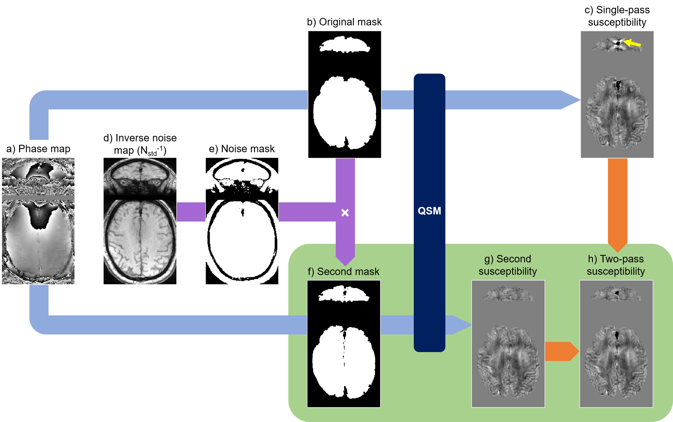
Quantitative Susceptibility Mapping (QSM) is an MRI technique with emerging clinical applications1. QSM calculates the tissue magnetic susceptibility from MRI phase images1-3. It aims to solve an ill-posed inverse problem often inducing streaking artifacts (Figure 1c, yellow arrow), particularly around extreme susceptibility values such as bleeds or calcifications. To suppress streaking, several studies have proposed variations on a two-pass masking approach4-6, i.e. performing QSM both with (Figure 1a-c) and without (Figure 1a,f-h) the extreme-susceptibility regions included in the tissue mask, and then combining the results (Figure 1h). However, these methods were designed for and integrated into specific QSM pipelines making them difficult to apply more broadly, focus on reducing streaking from blood vessels only, and/or require morphological operations that are sensitive to the location of extreme-susceptibility regions. Here we i) introduce a new, robust two-pass masking approach that is easy to implement and add to any QSM pipeline (optimised for the desired application), ii) demonstrate that this approach suppresses streaking artifacts around extreme-susceptibility regions such as interhemispheric calcifications which are quite common in elderly subjects, and iii) show, for the first time, that two-pass masking does not adversely affect susceptibility maps in subjects without extreme-susceptibility regions.Methods
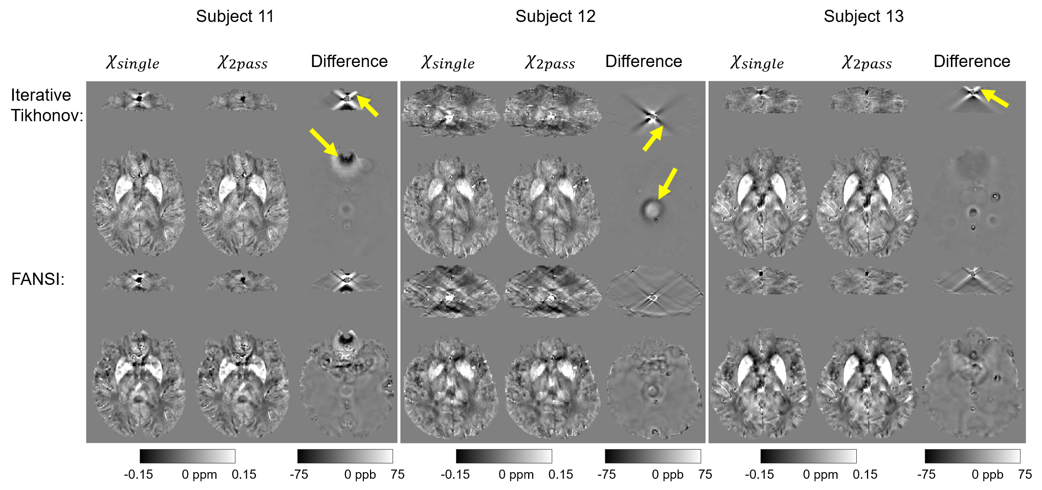
We used brain images from thirteen, 70-year-old subjects acquired for a clinical study7 at 3-Tesla (Biograph mMR, Siemens Healthineers, Erlangen, Germany) using a 3 minutes 48 seconds 3D GRE sequence and a 12-channel head coil with FOV=22×16.5×14.4 cm3, resolution=0.86×0.86×1.5 mm3, TEs=4.92/9.84/19.2 ms, BW=400/400/140 Hz/pix respectively, GRAPPA factor=2, TR=27 ms, and α=15°. Three of the thirteen subjects had large interhemispheric calcifications and one also had 1-cm-diameter intracerebral bleed.The first two, low-SNR echoes were necessary to perform accurate coil combination with ASPIRE8. Susceptibility maps were then calculated from the coil-combined, high-SNR, third-echo complex image using a (single-pass) QSM pipeline optimised for subjects without extreme susceptibility values: 1. phase unwrapping using ROMEO9, 2. background field removal using PDF10, and 3. susceptibility calculation using both iterative Tikhonov11,12 with α=0.02 and FANSI13,14 with α=5.2·10-5 optimised using L-curves and frequency masks15. Inverse noise maps (Nstd-1) for weighting in steps 2 and 3 were calculated from the multi-echo magnitude images16. Brain masks (Figure 1b) were created by applying SPM1217 to the last-echo magnitude image to segment and then merge GM, WM, and CSF, followed by three layers of Nstd-1-based mask erosion (i.e. removing voxels where Nstd-1<mean(Nstd-1)) around the brain edges. Images were rotated into the scanner frame after phase unwrapping18.
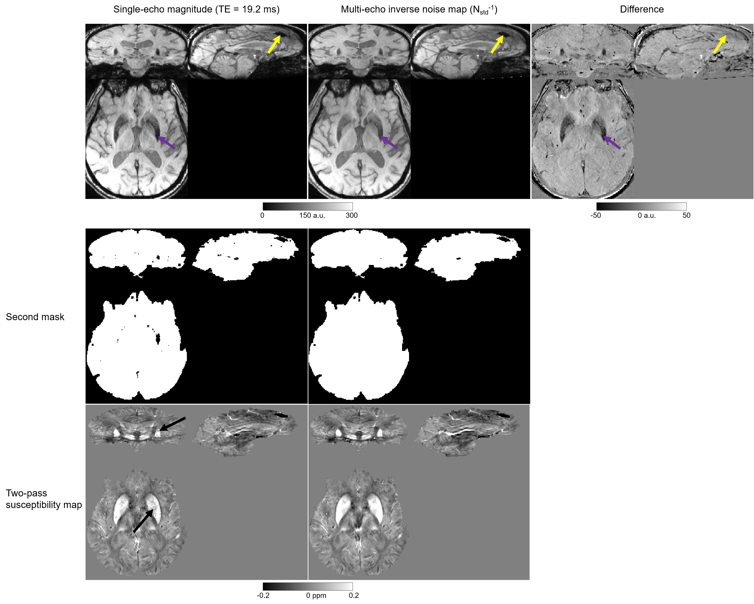
For the two-pass masking approach, steps 2 and 3 were repeated (Figure 1a,f-h) with a different (smaller) brain mask (Figure 1f) obtained by excluding high-noise regions, i.e. where Nstd-1<0.5·mean(Nstd-1), from the original mask throughout the whole brain (Figure 1b,d-f). Finally, a combined susceptibility map (Figure 1h) was created by superimposing the missing susceptibility values from the original, single-pass susceptibility map (Figure 1c) into the second susceptibility map (Figure 1g).
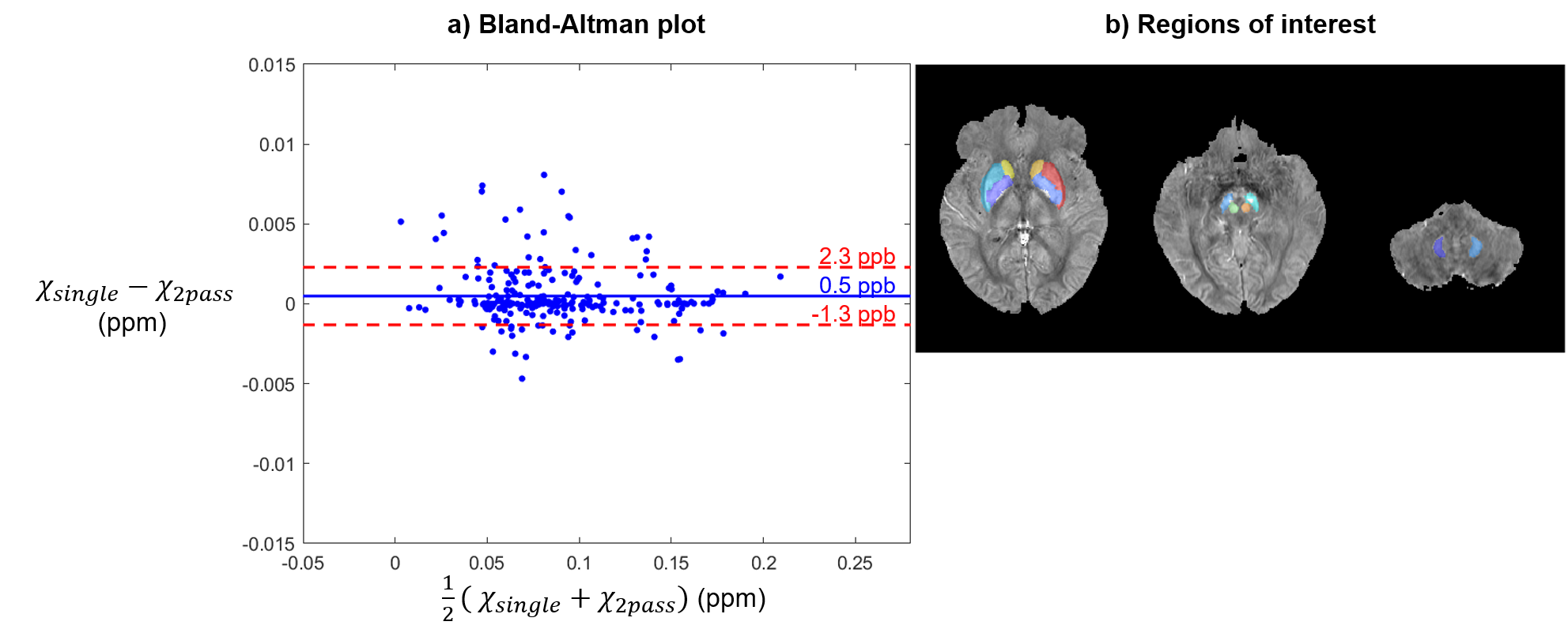
In the ten subjects without extreme-susceptibility sources, mean susceptibilities were calculated in twelve deep gray matter regions (Figure 4b) segmented using a multi-atlas tool19,20.
Results and Discussion
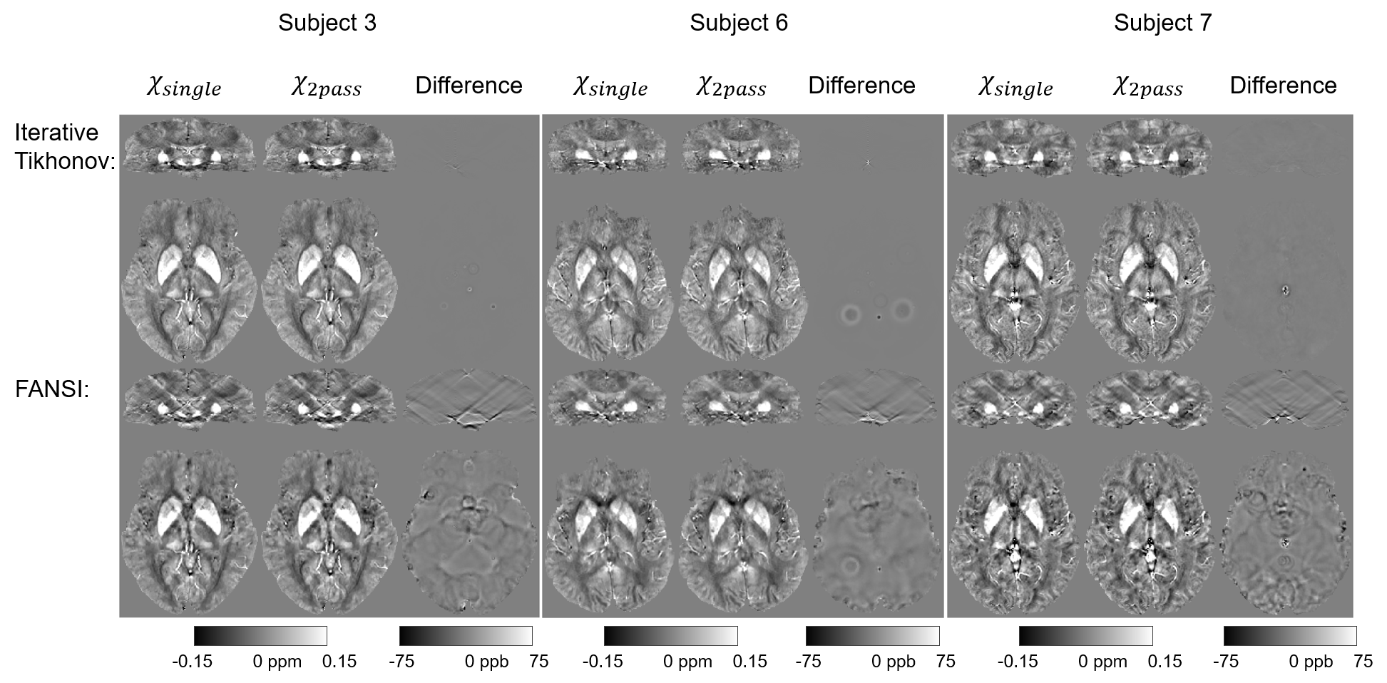
Figure 2 shows that this two-pass masking approach greatly reduces streaking artifacts around extreme-susceptibility regions (yellow arrows) in both the iterative Tikhonov and FANSI results. The difference images also confirm that two-pass masking does not remove any anatomical details. Figure 3 illustrates that two-pass masking does not affect the appearance of susceptibility maps in subjects without extreme-susceptibility sources; although the difference images show that it removes a few, subtle streaks, perhaps from blood vessels. The Bland-Altman plot (Figure 4a) of all segmented regions in the ten subjects without extreme-susceptibility sources shows that the susceptibility change induced by two-pass masking is negligible (between -1.3 and 2.3 ppb). This is corroborated by a (5.2±3.8) ppb root-mean-squared difference between the single-pass and two-pass susceptibility maps in these subjects.Our approach for implementing two-pass masking has several advantages over previous methods. It is easy to implement and integrate into any QSM pipeline (Figure 1, green box) by excluding voxels from an existing brain mask, and then performing QSM a second time with the new mask. Furthermore, the method for creating the second brain mask is flexible and can be designed for a specific application or anatomical region. If multi-echo images are available, we recommend creating the mask by thresholding the multi-echo Nstd-1 (Figure 1b,d-f) rather than the magnitude as the latter is echo-time dependent and using it can lead to artifacts (Figure 5). Note that two-pass masking requires the calculation of the single-pass susceptibility map making the two-pass susceptibility map an additional output rather than a replacement. Consequently, there is no risk in adding two-pass masking to QSM pipelines in large, clinical studies. Although we focused on brain images, two-pass masking may be applicable outside of the brain to suppress streaking from e.g. calcifications and fatty fascia.
Conclusions
Two-pass masking greatly reduced streaking artifacts around extreme-susceptibility regions, which are particularly common in the brains of elderly subjects, without affecting other anatomical features in the susceptibility map. Our method for two-pass masking is easy to add to any QSM pipeline without any risk as the two-pass susceptibility map is an additional output rather than a replacement of the original, optimised susceptibility map.Acknowledgements
We thank Prof. Jonathan Schott for permission to use images acquired as part of Insight 46, a neuroscience sub-study of the MRC National Survey of Health and Development, to demonstrate our two-pass masking approach. Karin Shmueli and Anita Karsa were supported by European Research Council Consolidator Grant DiSCo MRI SFN 770939References
1. Eskreis‐Winkler, Sarah, et al. "The clinical utility of QSM: disease diagnosis, medical management, and surgical planning." NMR in Biomedicine 30.4 (2017).
2. Reichenbach, J. R., et al. "Quantitative susceptibility mapping: concepts and applications." Clinical neuroradiology 25.2 (2015): 225-230.
3. Wang, Yi, and Tian Liu. "Quantitative susceptibility mapping (QSM): decoding MRI data for a tissue magnetic biomarker." Magnetic resonance in medicine 73.1 (2015): 82-101.
4. Wei, Hongjiang, et al. "Streaking artifact reduction for quantitative susceptibility mapping of sources with large dynamic range." NMR in Biomedicine 28.10 (2015): 1294-1303.
5. Yaghmaie, Negin, et al. "QSMART: Quantitative susceptibility mapping artifact reduction technique." NeuroImage 231 (2021): 117701.
6. Stewart, Ashley Wilton, et al. "QSMxT: Robust Masking and Artefact Reduction for Quantitative Susceptibility Mapping." bioRxiv (2021).
7. Lane, Christopher A., et al. "Study protocol: Insight 46–a neuroscience sub-study of the MRC National Survey of Health and Development." BMC neurology 17.1 (2017): 1-25.
8. Eckstein, Korbinian, et al. "Computationally efficient combination of multi‐channel phase data from multi‐echo acquisitions (ASPIRE)." Magnetic resonance in medicine 79.6 (2018): 2996-3006.
9. Dymerska, Barbara, et al. "Phase unwrapping with a rapid opensource minimum spanning tree algorithm (ROMEO)." Magnetic Resonance in Medicine 85.4 (2021): 2294-2308.
10. Liu, Tian, et al. "A novel background field removal method for MRI using projection onto dipole fields." NMR in Biomedicine 24.9 (2011): 1129-1136.
11. Karsa, Anita, Shonit Punwani, and Karin Shmueli. "An optimized and highly repeatable MRI acquisition and processing pipeline for quantitative susceptibility mapping in the head‐and‐neck region." Magnetic Resonance in Medicine 84.6 (2020): 3206-3222.
12. https://xip.uclb.com/product/mri_qsm_tkd
13. Milovic, Carlos, et al. "Fast nonlinear susceptibility inversion with variational regularization." Magnetic resonance in medicine 80.2 (2018): 814-821.
14. https://gitlab.com/cmilovic/FANSI-toolbox/
15. Milovic, Carlos, et al. "Comparison of parameter optimization methods for quantitative susceptibility mapping." Magnetic resonance in medicine 85.1 (2021): 480-494.
16. Kressler, Bryan, et al. "Nonlinear regularization for per voxel estimation of magnetic susceptibility distributions from MRI field maps." IEEE transactions on medical imaging 29.2 (2009): 273-281. (Equation 14)
17. Ashburner, John, et al. "SPM12 manual." Wellcome Trust Centre for Neuroimaging, London, UK 2464 (2014).
18. Kiersnowski, Oliver C., et al. "The Effect of Oblique Image Slices on the Accuracy of Quantitative Susceptibility Mapping and a Robust Tilt Correction Method." ISMRM & SMRT Annual Meeting & Exhibition, 2021.
19. Li, Xu, et al. "Multi-atlas tool for automated segmentation of brain gray matter nuclei and quantification of their magnetic susceptibility." Neuroimage 191 (2019): 337-349.
20. https://braingps.mricloud.org/
Figures