2453

Adaptive k-Space Sampling in Magnetic Resonance Imaging Using Reinforcement Learning

Edith Franziska Baader¹, Fabian Theißen¹, Nicola Pezzotti^2,3, and Volkmar Schulz^1,4,5,6
¹Department of Physics of Molecular Imaging Systems, Institute for Experimental Molecular Imaging, RWTH Aachen University, Aachen, Germany, ²Philips Research, Eindhoven, Netherlands, ³Department of Mathematics and Computer Science, Eindhoven University of Technology, Eindhoven, Netherlands, ⁴Physics Institute III B, RWTH Aachen University, Aachen, Germany, ⁵Fraunhofer Institute for Digital Medicine MEVIS, Bremen, Germany, ⁶Hyperion Hybrid Imaging Systems GmbH, Aachen, Germany

Synopsis

One approach to accelerate MRI scans is to acquire fewer k-space samples. Commonly, the sampling pattern is selected before the scan, ignoring the sequential nature of the sampling process. A field of machine learning addressing sequential decision processes is reinforcement learning (RL). We present an approach for creating adaptive two-dimensional (2D) k-space trajectories using RL and the so-called action space shaping. The trained RL algorithm adapts to a variety of basic 2D shapes outperforming simple baseline trajectories. By shaping the action space of the RL agent we achieve better generalization and interpretability of the agent.

Introduction

One approach to accelerate MRI scans is to acquire fewer k-space samples. Commonly, the k-space sampling pattern is determined by the selected scan. However, the sampling trajectory of the k-space in MRI can be considered as a sequential decision process in which the amount of information increases with each acquired sample. A field of machine learning addressing sequential decision processes is reinforcement learning (RL). The learner, called the agent in RL, interacts with an environment aiming at maximizing the cumulative reward. The interaction is divided into discrete time steps at which the agent chooses an action based on the information provided by the environment¹.
Previous research on adaptive sampling approaches focuses on choosing the next k-space line in Cartesian readout schemes^2-7. Here, we present an approach for creating adaptive 2D k-space trajectories using reinforcement learning (RL) and action space shaping⁸ which gives a high interpretability of the agent.

Methods

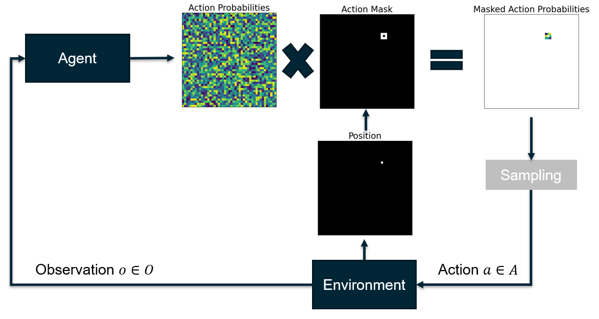
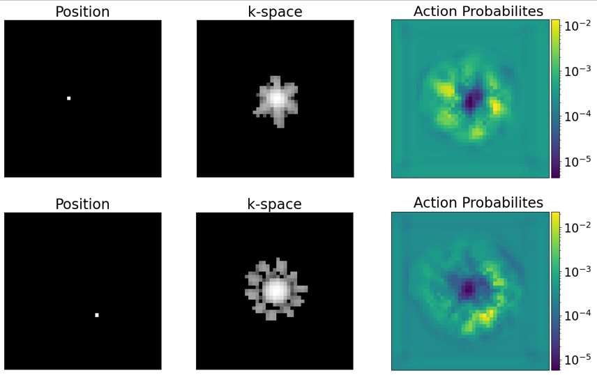
The RL environment is characterized by the following elements:

Observation space: The agent receives at every time step the current position in k-space and the zero-filled absolute-valued k-space in logarithmic scale.
Action space: The action space has the same size as the k-space. Thus, a probability is assigned to every k-space pixel regardless of whether selecting this pixel is a valid action as defined by our action space shaping approach.
Action space shaping: We constrain the agent to create connected trajectories by only considering sampling neighboring pixels of the current position as valid actions and masking out all other actions (Fig. 1). We use the action masking implementation of Tang et al.⁹.
Initial state: The agent starts every trajectory at the center of the k-space.
Terminal state: One trajectory ends after 200 time steps, which were chosen here as the maximum number of samples. This allows the agent to sample up to ∼10% of k-space.
Reward function: The reward is the L2 distance of the reconstructed images at two consecutive time steps. The image is reconstructed using an inverse fast Fourier transform of the zero-filled k-space.

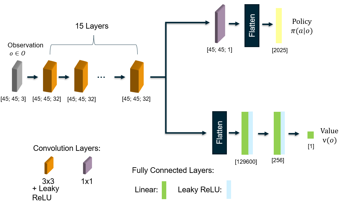
For the implementation of the environment, we use the toolkit Open AI Gym¹⁰. For the agent, we use a custom policy network (Fig. 2) and the adaptation of Tang et al.⁹ of the implementation of the proximal policy optimization algorithm PPO2 provided by the package Stable Baselines¹².
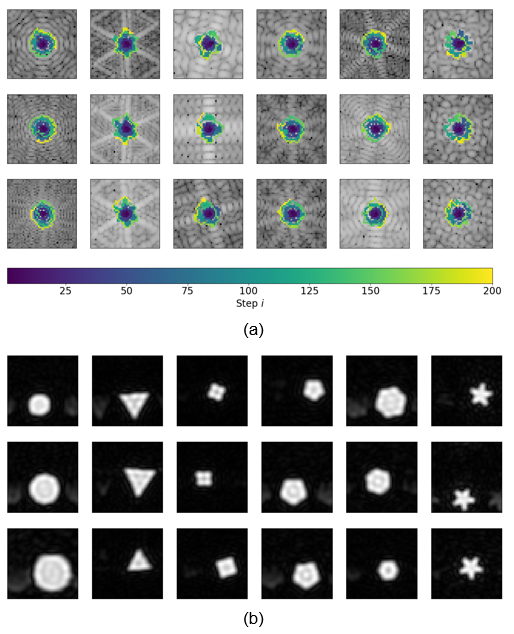
The agent is trained for 50 million time steps with a set of 18 simulated k-spaces of size 45x45 using phantoms of basic geometric shapes generated by an adaptation of the geometric shapes generator proposed by El Korchi et al.¹³. The simulation is performed using the package Virtual Scanner¹⁴ and its echoplanar imaging sequence. After training, the agent is tested on a set of unknown k-spaces and the trajectories are created deterministically meaning that always the action with the highest probability is selected.

Results

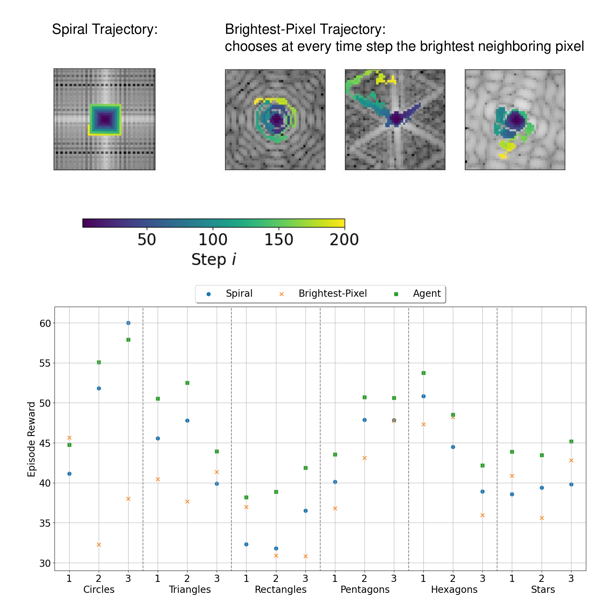
The agent’s trajectories differ depending on the presented k-space and cover characteristic bright patterns in the k-space center (Fig. 3). The episode reward of the agent’s trajectories is higher than simple baseline trajectories for almost all samples in the test set (Fig. 4). The visualization of the action probabilities before the masking operation shows that the probability for sampling a specific k-space pixel decreases after having been sampled (Fig. 5). Furthermore, the action probability is high for some locations that continue the characteristic bright pattern of the k-space.

Discussion

The agent adapts its trajectories to unknown k-spaces during acquisition. Giving the agent one action for every k-space pixel and enforcing constraints on the trajectory via action space shaping gives a high interpretability of the trajectory creation by the agent.
Furthermore, the constraints on the k-space trajectory can be adapted straightforwardly by changing the action mask. For example, to speed up the acquisition, valid k-space pixels might be at a certain radius from the current position and the trajectory is continued by a straight line to this pixel. This is possible thanks to our action space shaping approach, in which the probabilities are computed for all k-space pixels.

Conclusion

The results show that an RL agent can reasonably adjust k-space trajectories during acquisition. Our presented action space shaping approach gives insight into the reasoning of the agent during trajectory creation. Next steps include combining the agent with a trainable reconstruction and testing the approach on clinical data.

Acknowledgements

No acknowledgement found.

References

1. Sutton R S, Barto A G. Reinforcement learning: an introduction. The MIT Press, second edition; 2018

2. Bakker T, van Hoof H, Welling M. Experimental design for MRI by greedy policy search. arXiv:2010.16262. 2020.

3. Jin K H, Unser M, Yi K M. Self-supervised deep active accelerated MRI. arXiv:1901.04547. 2019.

4. Pineda L et al. Active MR k-space sampling with reinforcement learning. MICCAI 2020; pp 23-33.

5. Walker-Samuel S. Using deep reinforcement learning to actively, adaptively and autonomously control a simulated MRI. ISMRM 2019.

6. Zhang Z et al. Reducing uncertainty in undersampled MRI reconstruction with active acquisition. 2019 IEEE/CVF CVPR. 2019; pp 2049-2053.

7. Yin T et al. End-to-end sequential sampling and reconstruction for MR imaging. arXiv:2105.06460. 2021.

8. Kanervisto A, Scheller C, Hautamäki V. Action Space Shaping in Deep Reinforcement Learning. 2020 IEEE CoG. 2020; pp 479-486.

9. Tang C-Y, Liu C-H, Chen W-K, You S D. Implementing action mask in proximal policy optimization (PPO) algorithm. ICT Express. 2020; 6(3):200-203.

10. Brockman G et al. Openai gym. arXiv:1606.01540. 2016.

11. Mnih V et al. Asynchronous Methods for Deep Reinforcement Learning. arXiv:1602.01783. 2016.

12. Hill A et al. Stable Baselines. https://github.com/hill-a/stable-baselines; 2018.

13. El Korchi A, Ghanou Y. 2D geometric shapes dataset - for machine learning and pattern recognition. Data in Brief. 2020; 32:106090.

14. Tong G et al. Virtual scanner: MRI on a browser. Journal of Open Source Software. 2019; 4(43):1637.

Figures

Figure 1. Concept of our action space shaping: the agent outputs a probability for every action (here every k-space pixel). Element-wise multiplication of this probability map by a binary mask given by the environment masks all invalid actions out; the action is then sampled from the valid action probabilities (here the neighboring k-space pixels of the current position).

Figure 2. Sketch of the custom policy network with actor-critic architecture¹¹. The first input channel of the network is the position and the second and third channel the k-space. The joint part of the network consists of 15 convolutional layers with filter size 3x3. In the policy branch, the resulting feature maps are mapped by a 1x1 convolution to the action probability map. Hence, the action probabilities are computed using only convolutional layers conserving the size of the k-space.

Figure 3. Trajectories created by the trained agent on the test set (a) and corresponding reconstructed images (b). The color in (a) encodes the order in which the k-space pixels are sampled. The images are reconstructed using an inverse fast Fourier transform of the zero-filled k-space. The trajectories focus on characteristic bright patterns in the k-space center (a).

Figure 4. Comparison of the episode rewards (cumulative reward collected throughout one episode) of the agent’s trajectories (Fig. 3) with two simple baseline trajectories.

Figure 5. Two examples of action probability maps of different episodes at 115 time steps (top) and 181 time steps (bottom). The probability of k-space pixels that are already acquired is lower than for unknown k-space pixels that are close to acquired pixels. Furthermore, the action probability is high for some characteristic parts of the k-space pattern. Note that we achieve a probability map thanks to the use of the action space shaping we introduce in this work.

Proc. Intl. Soc. Mag. Reson. Med. 30 (2022)

2453

DOI: https://doi.org/10.58530/2022/2453