Introduction

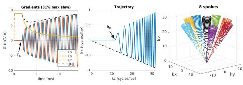
Short T2 imaging uses an echo time (TE) of close to zero, which is only attainable with center-out non-Cartesian trajectories. Unfortunately the center-out radial trajectory is unfavorable in terms of sampling efficiency and produces non-uniform coverage of k-space, which leads to a strong dependence of the point spread function (PSF) on number of spokes (N). Density adapted and cones trajectories improve the sampling efficiency [1-3] by lengthening the readout duration to produce more uniform k-space coverage and fulfill the Nyquist criterion with fewer spokes.

A variant of cones referred to in Ref 1 as constant polar angle constant sample density (and in the present study as corkscrew) is represented in Figure 1. To quickly escape the densely sampled center of k-space, the trajectory traverses radially to a specified radius (k₀) then switches to a density adapted waveform with slower traversal in the radial direction and a spiral motion in the orthogonal plane. There are several design choices associated with this trajectory; the purpose of the present study is to derive optimal (or, at least, reasonable) parameter values based on geometrical considerations.

Theory

1.1. Nyquist number of spokes for radial
Tessellating a sphere of radius k_max using n-sided regular polygons of surface area a requires N = 4πk_max² / a polygons. If spoke endpoints are situated at the polygon centers then the Nyquist criterion requires the distance between neighboring spokes (equal to 2 times the apothem) to be 1, in units of inverse field of view (fov^-1). Since a = n / 4πtan(π/n), the required number of spokes is:

N = 16πk_max² / n tan(π/n)

The value π matrix² (n=4) is commonly used [4-5].

1.2. Sub-Nyquist sampling
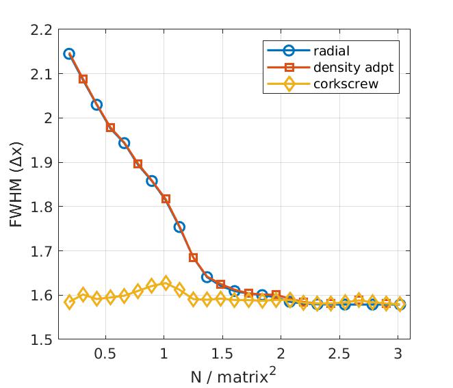
Practical scan times limit N to values well below Nyquist. E.g. for an imaging matrix of 128, Eq 1 requires ~50000 spokes. With fewer spokes, some aliasing is to be expected but numerical simulations also reveal a large change in the PSF. An approximately linear decrease in full width at half maximum (FWHM) is observed with N (Figure 2) until it reaches the theoretical minimum of 1.59 times the nominal voxel size [6]. For the corkscrew trajectory, the dependence is much weaker and can be neglected for practical purposes.

1.3. Choice of k0
A reasonable criterion for k₀ is the point where the distance between spokes is 1 (in units of fov^-1). Beyond this point the Nyquist spacing is no longer satisfied so it is a natural point to switch to the corkscrew or density adapted trajectory. This leads to k₀ = sqrt( n tan(π/n) N / 16π ) or assuming n=4:

k₀ = sqrt( N / 4π)


1.4. Corkscrew
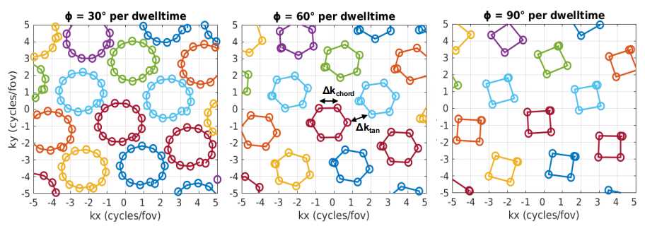
At k₀ the tangential distance (Δk_tan) between spokes is by definition 1, which makes it a natural point to change trajectory. The corkscrew seeks to reduce Δk_tan at k_max by distributing points around a circle of radius r with angular spacing Φ (see Figure 3), effectively reducing it to k_max / k₀ - 2r. While r and Φ are nominally free parameters, it is possible to make reasonable choices based on theoretical considerations:

i. The distance between points on the same spoke decreases rapidly after k₀ (see Figure 1) and may be approximated by the chord length:

Δk_chord = 2r sin(Φ/2)

ii. Equal spacing between points on neighboring spokes may be achieved by setting Δk_tan = Δk_chord. With (i) this yields a target radius for the corkscrew:

r = (1+sin(Φ/2))^-1 k_max / 2k₀

iii. Expressing the Nyquist criterion as Δk_tan = Δk_chord = 1 leads to a target value for the angular rate as a function of N (for n = 4):

Φ = 2 acsc( sqrt(π/N) matrix - 1 )

which evaluates to 53.8° for the example in Figure 3.

1.6. Angular rotation rate
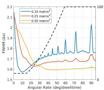
The FWHM was numerically simulated from Φ = 0 to 90° for different numbers of spokes. Results in Figure 4 indicate that the FWHM passes through minima at different values of Φ depending on N, and also exhibits evidence of peak structure. Neighboring loops of the corkscrew effectively overlap when the distance between them is less than 1 and the optimal Φ arranges points to minimize redundancy in filling k-space. Peaks at 60, 72, 90° etc. indicate that the overlap is unfavorable whenever 360/Φ is a small integer.

This can be recognized in Figure 3 where the first and last points are almost coincident and hence redundant. Overlaid on the plot (dashed line) is the gradient slew rate as a percentage of the maximum hardware specification.

1.6. Nyquist number of spokes for corkscrew
The expression in Section 1.4(iii) can be rearranged to give an estimate for the Nyquist number of spokes for corkscrew (for n = 4).

N = [ sin(Φ/2) / (1+sin(Φ/2)) ]² π matrix²

This evaluates to around 0.13 matrix² or 2200 spokes for a matrix of 128. This is substantially lower than the ~50000 spoke for radial sampling and in qualitative agreement with simulation results (Figure 2).

Discussion

Protocol design with non-Cartesian trajectories involves making choices for sometimes unfamiliar sequence parameters. Theoretical justifications can support specific choices and help standardize imaging protocols for sodium and other rapidly decaying signals [7].

Acknowledgements

No acknowledgement found.