2445
Calibration kernels with Alternative Sampling Scheme (CASS) for Parallel Imaging: SENSE meets CASS1Department of High-field Magnetic Resonance, Max Planck Institute for Biological Cybernetics, Tuebingen, Germany, 2Graduate Training Centre of Neuroscience, University of Tuebingen, Tuebingen, Germany, 3Department of Biomedical Magnetic Resonance, University of Tuebingen, Tuebingen, Germany, 4Athinoula A. Martinos Center for Biomedical Imaging, Department of Radiology, Harvard Medical School, Massachusetts General Hospital, Charlestown, MA, United States
Synopsis
We developed new calibration kernels with an alternative undersampling scheme (CASS) for parallel imaging to reduce coherent aliasing artifacts and noises. By sampling k-space lines with irregular and blockwise patterns, incoherent aliasing patterns and noise signals were spread in reconstructed CASS images. Noteworthily, the CASS method outperformed the conventional GRAPPA method at higher acceleration factors.
Introduction
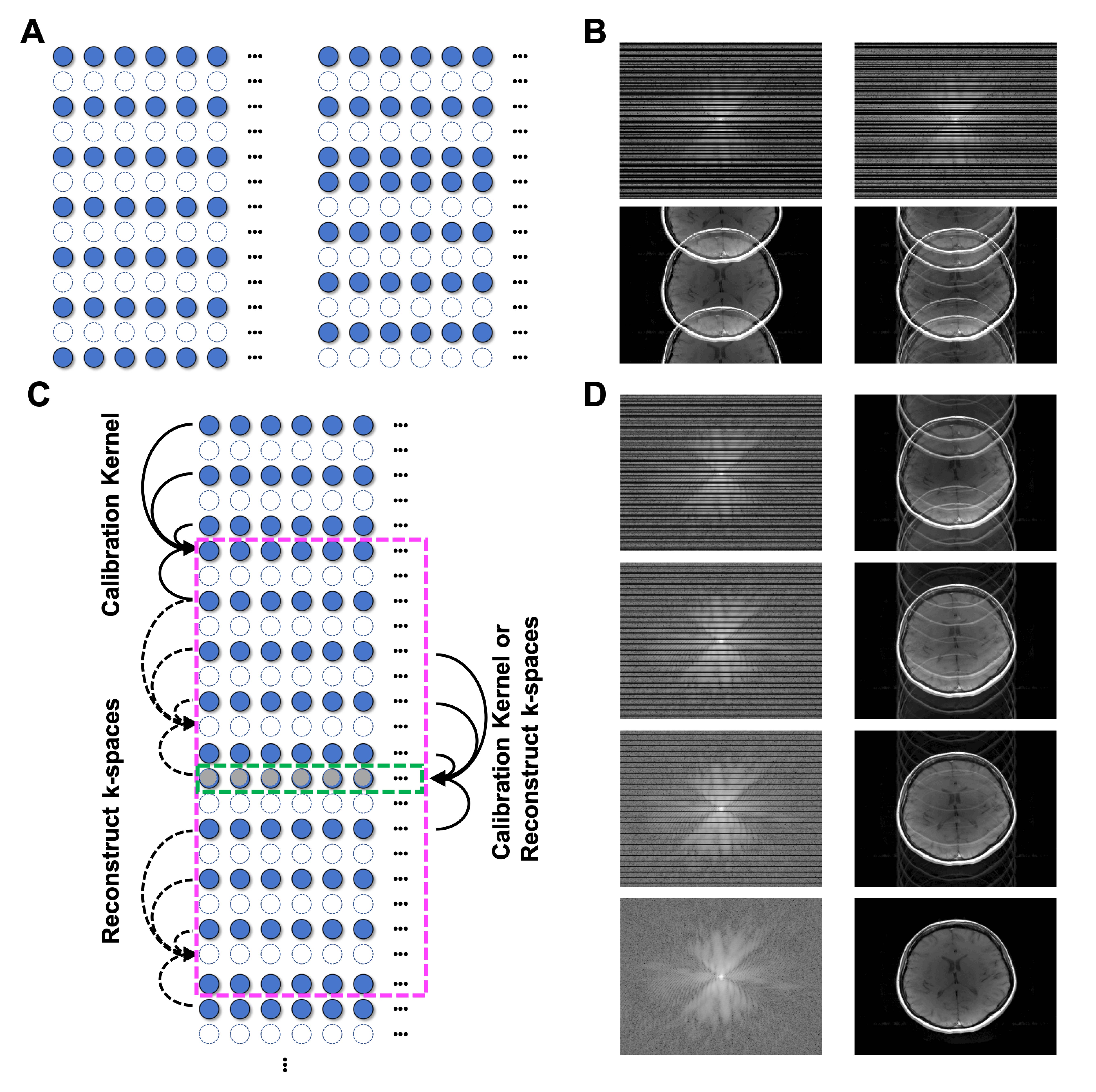
Parallel Imaging (PI)1-5 has successfully provided acceleration methods to reduce scan time in human studies and clinical applications. Since Generalized Autocalibrating Partially Parallel Acquisitions (GRAPPA)2 and SENSitivity Encoding (SENSE)3 have been developed, extensive efforts were made to improve the performance of GRAPPA and SENSE in terms of noise amplification and aliasing artifacts by using technical advances in multi-channel receive coils6 and mathematical models7-9. Nevertheless, to date mostly the regular undersampling schemes are used in PI, additionally acquiring autocalibration signals (ACS) for GRAPPA or reference signals for SENSE. Here, we developed an irregular and alternative undersampling scheme to reduce coherent aliasing artifacts and noise amplification. Using acceleration factors (AF) of 2 and 3, we applied calibration kernels with an alternative sampling scheme (CASS) without additional ACS and reconstructed multi-slice images without severe coherent aliasing artifacts, demonstrating spreading incoherent noise and aliasing patterns in difference images. With central k-space signals, we generated variable alternative undersampling patterns (i.e., dense in center and sparse in peripheral k-spaces) mimicking the energy distribution of k-space10. Notably, the CASS method outperformed the conventional GRAPPA method for the same net AFs, showing reduced high-frequency noises and invisible coherent aliasing artifacts in reconstructed images. Thus, our work provides a robust and stable PI method to reliably preserve anatomical information with CASS.Methods
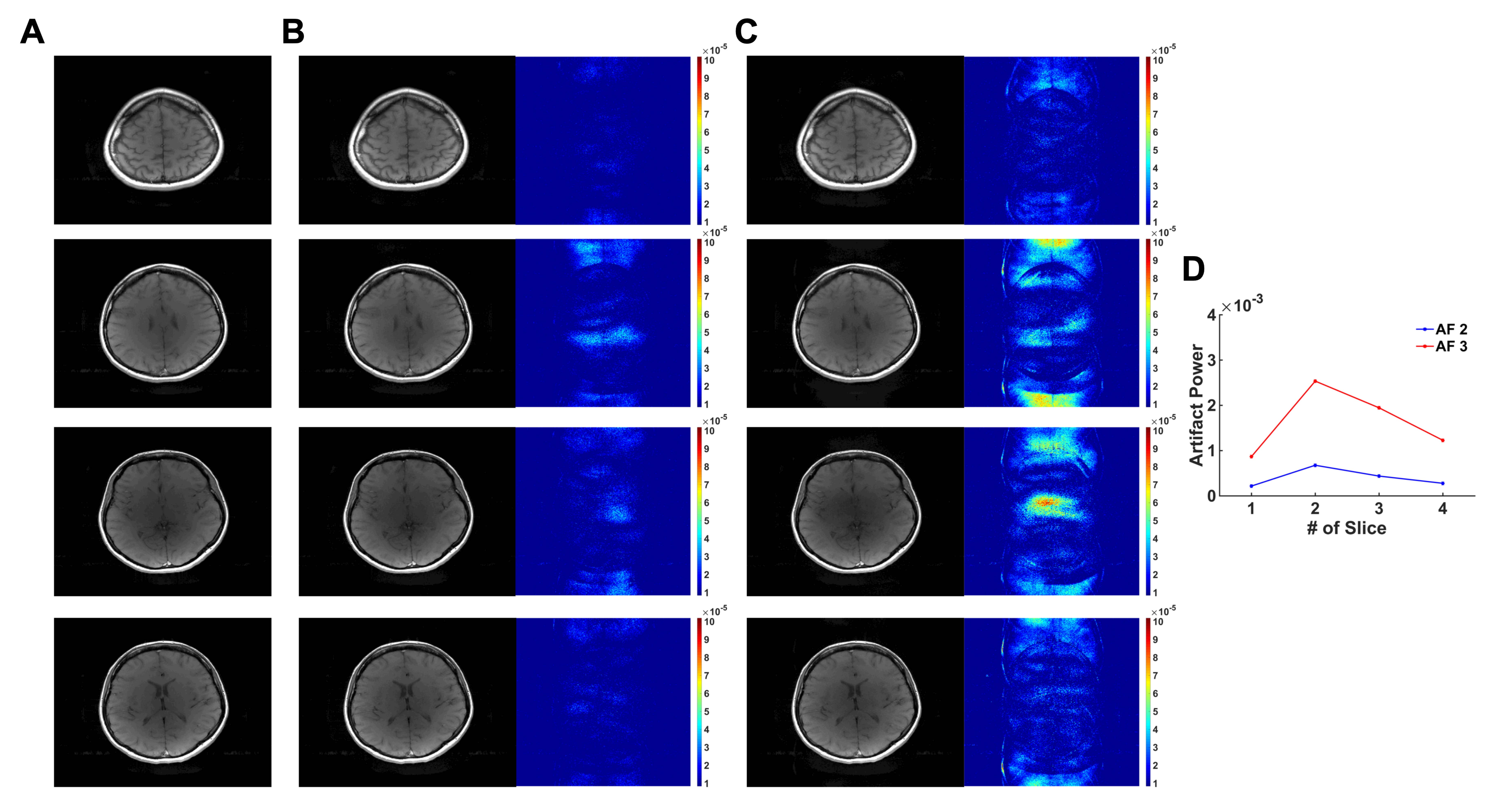
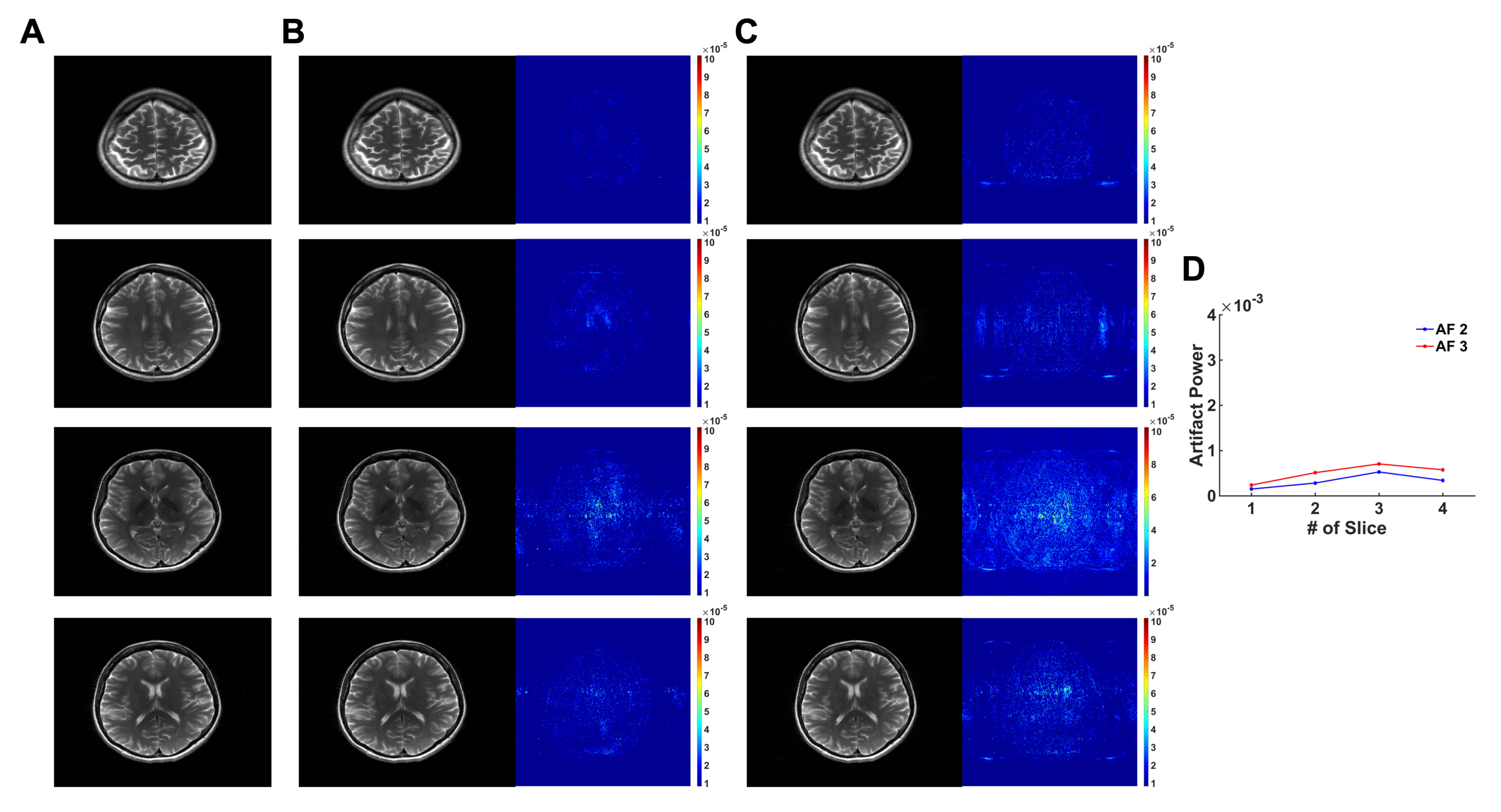
Data Acquisition: T1-weighted SE and T2-weighted TSE datasets were acquired without acceleration in a healthy subject using 64 receiver coils at a Siemens 3T MRI system. The following parameters were used: FOV 256 x 256 mm2, matrix 256 x 256, slice thickness 4 mm, number of slices 4, for SE, TR/TE 600/9.6 ms, TA 2 min 35 sec, for TSE, TR/TE 6000/100 ms, turbo factor 15, and TA 1 min 56 sec.Reconstruction: Full-sampled datasets were retrospectively undersampled by using a regular sampling scheme (Fig. 1A, left) for GRAPPA and using irregular (i.e., any sampling patterns with/without central k-space lines and/or high-frequency k-space lines, Fig. 1C and 4A-C, right) and alternative sampling schemes (Fig. 1A, right) for CASS. For GRAPPA2, undersampled k-spaces were reconstructed using ACS (24, 32, 10 lines for AF 1.8, 2.4, 2.8, respectively). For CASS, we sampled odd and even numbers of one block (Fig. 1C, dashed box) and divided a whole k-space with multiple blocks. Then, we calculated calibration kernels and reconstructed block-by-block missing k-spaces which have the same harmonics in turns (Fig. 1C and 1D). To better estimate calibration kernels in low and high-frequency regions of k-space, we divided a whole k-space into sub-blocks (e.g., 2 sub-blocks for AF 2, 5 sub-blocks for AF 3) and used adjacent signals within a block to calculate calibration kernels. To compare the performance of CASS with GRAPPA, we added central k-space signals and reconstructed missing k-space lines with blockwise calibration kernels (e.g., 2 kernels for AF 2 and 5 kernels for AF 3, corresponding to the number of sub-blocks) and calculated artifact powers (AP)11 instead of g-factor maps12 because we obtained difference images from full-sampled reference images. All data analyses were implemented in Matlab software (Mathworks, Natick, MA).
Results
The CASS method reliably reconstructed multi-slice T1 and T2 images that were respectively undersampled with AF 2 and AF 3 (Fig. 2 and 3) following the blockwise reconstruction processing (Fig. 1C and 1D). In individual slices, the reconstruction performances were acceptable, showing invisible coherent aliasing artifacts and spreading incoherent noise pattens (Fig. 2B, 2C, 3B, and 3C). However, some of the reconstructed T1-weighted images had relatively high noise amplification in AF 3 (Fig. 2C) whereas T2-weighted images of the same slice had less noise amplification, possibly indicating contaminated k-space along the phase-encoding direction due to subject motion during the T1-weighted acquisition. Except for those T1-weighted images, all the reconstructed images had low and similar AP values (background noise level, Fig. 2D and 3D). To further investigate the performance of the CASS method, we compared CASS (including central k-space lines) with GRAPPA (Fig. 4). Indeed, CASS and GRAPPA showed similar performances and image quality in net AF 1.8 and 2.4 (Fig. 4D, 4E, 4G, and 4H). Noteworthily, in net AF 2.8, the CASS (Fig. 4I) outperformed the GRAPPA (Fig. 4F), demonstrating reduced noise amplification and coherent aliasing artifacts in difference images whereas the GRAPPA image had severe coherent aliasing artifacts and higher AP value (Fig. 4J).Discussion and Conclusion
Using our new CASS method, we reliably reconstructed anatomical multi-slice images with net AF 1.8 to 3. In contrast to the existing regular sampling PI methods1-5, the CASS method could be applied in AF 2 and 3 without acquiring additional ACS, indicating potentials to avoid problems caused by mismatches between reference scan and main acquisition in SENSE3 and Echo Planar Imaging13. Moreover, CASS outperformed GRAPPA in higher AF, having variable sampling patterns that mimick the energy distribution of k-space10. Thus, we have demonstrated the robustness and stability of CASS with multiple AFs. Furthermore, the CASS method can also be improved by incorporating advanced mathematical models, e.g., L2 regularization13, low-rank approximation14, and L1 optimization (e.g., compressed sensing)15, similar to advanced GRAPPA studies. For 3D PI, the CASS method can be easily applied by alternatively undersampling data in phase- and slice-encoding dimensions.Acknowledgements
This research was supported by the German Research Foundation (DFG) Yu215/3-1, BMBF 01GQ1702, and the internal funding from Max Planck Society.References
1 Sodickson, D. K. & Manning, W. J. Simultaneous acquisition of spatial harmonics (SMASH): fast imaging with radiofrequency coil arrays. Magn Reson Med. 38 (4), 591-603, (1997).
2 Griswold, M. A. et al. Generalized Autocalibrating Partially Parallel Acquisitions (GRAPPA). Magnetic Resonance in Medicine. 47 (6), 1202-1210, (2002).
3 Pruessmann, K. P., Weiger, M., Scheidegger, M. B. & Boesiger, P. SENSE: Sensitivity encoding for fast MRI. Magnetic Resonance in Medicine. 42 (5), 952-962, (1999).
4 Breuer, F. A. et al. Controlled aliasing in parallel imaging results in higher acceleration (CAIPIRINHA) for multi-slice imaging. Magn Reson Med. 53 (3), 684-691, (2005).
5 Blaimer, M. et al. SMASH, SENSE, PILS, GRAPPA: how to choose the optimal method. Top Magn Reson Imaging. 15 (4), 223-236, (2004).
6 Keil, B. et al. A 64-channel 3T array coil for accelerated brain MRI. Magn Reson Med. 70 (1), 248-258, (2013).
7 Zhao, T. & Hu, X. Iterative GRAPPA (iGRAPPA) for improved parallel imaging reconstruction. Magn Reson Med. 59 (4), 903-907, (2008).
8 Lustig, M. & Pauly, J. M. SPIRiT: Iterative self-consistent parallel imaging reconstruction from arbitrary k-space. Magn Reson Med. 64 (2), 457-471, (2010).
9 Park, S. & Park, J. Adaptive self-calibrating iterative GRAPPA reconstruction. Magn Reson Med. 67 (6), 1721-1729, (2012).
10 Sheng, J., Shi, Y. & Zhang, Q. Improved parallel magnetic resonance imaging reconstruction with multiple variable density sampling. Sci Rep. 11 (1), 9005, (2021).
11 Park, J., Larson, A. C., Zhang, Q., Simonetti, O. & Li, D. High-resolution steady-state free precession coronary magnetic resonance angiography within a breath-hold: parallel imaging with extended cardiac data acquisition. Magn Reson Med. 54 (5), 1100-1106, (2005).
12 Breuer, F. A. et al. General formulation for quantitative G-factor calculation in GRAPPA reconstructions. Magn Reson Med. 62 (3), 739-746, (2009).
13 Liu, W., Tang, X., Ma, Y. & Gao, J. H. Improved parallel MR imaging using a coefficient penalized regularization for GRAPPA reconstruction. Magn Reson Med. 69 (4), 1109-1114, (2013).
14 Shin, P. J. et al. Calibrationless parallel imaging reconstruction based on structured low-rank matrix completion. Magn Reson Med. 72 (4), 959-970, (2014).
15 Otazo, R., Kim, D., Axel, L. & Sodickson, D. K. Combination of compressed sensing and parallel imaging for highly accelerated first-pass cardiac perfusion MRI. Magn Reson Med. 64 (3), 767-776, (2010).
Figures