2441
Comparison between GRAPPA and automatic compressed sensing-based reconstruction up to 16-fold acceleration1Centre for Functional and Metabolic Mapping (CFMM) | Robarts Research Institute | Western University, London, ON, Canada, 2Department of Medical Biophysics | Schulich School of Medicine and Dentistry | Western University, London, ON, Canada, 3Aix-Marseille Universite | CNRS | CRMBM, Marseille, France, 4Siemens Healthcare Limited, Oakville, ON, Canada
Synopsis
With the recent development of an automatic compressed sensing (CS)-based reconstruction method, we investigated its allowance to recover T2* maps from prospectively undersampled multi-echo, gradient echo-based acquisitions at 7T. We compared our CS method with the more conventional GRAPPA-based reconstruction using up to 16-fold acceleration. In contrast to GRAPPA, our CS-based method allows recovery of T2* maps up to 16-fold acceleration, which demonstrates its promise for ultra-fast acquisitions. However, current results also show some caveats that need to be addressed as future work.
Purpose
To design a prospective and automatic reconstruction pipeline based on compressed sensing to allow reliable extraction of T2* maps from ultra-fast, multi-echo gradient-echo (ME-GRE) acquisitions.Introduction
Compressed sensing (CS) MRI reconstruction1–3 can be described as,$$\hat{x}=\textrm{argmin}_x\hspace{2mm}\|Ax-y\|_2^2+\lambda\|\Psi x\|_1,\hspace{6mm}\textrm{(1)}$$
where the data consistency (first term of Eq.(1)) makes the reconstruction, $$$x$$$, to resemble the acquired k-space data, $$$y$$$, after the net operator, $$$A$$$. The regularizer (second term) imposes sparsity from the reconstruction. One of the problems of using Eq. (1), is determining the regularization weighting, $$$\lambda$$$. An incorrect $$$\lambda$$$ generates significant image degradation. We recently presented a novel CS-based reconstruction with automatic selection of the regularization weighting to streamline this process4. Therefore, evaluation of the applicability of these reconstructions from ultra-fast acquisitions to extract biomarkers such as T2* is the next vital step. As such, we explored the limits of our reconstruction and its advantages over GRAPPA, in terms of the estimation of T2*.
Methods
Acquisition & ReconstructionWe acquired 4 subjects on a investigational 7T MRI scanner (MAGNETOM 7T Plus, Siemens Healthcare, Erlangen, Germany) with a head-only gradient system and an in-house built 32-channel receive and 8-channel transmit head coil5. For each subject, we acquired one fully sampled (non-accelerated) 3D ME-GRE sequence as reference for comparing reconstructions, using the following acquisition parameters: FOV= 208x208x208 mm; isotropic spatial resolution= 1 mm; TE0/TEΔ/TR= 2.54/2.16/20 ms and 5 echoes; total acquisition time 14:25. Then, we acquired 6 prospectively undersampled 3D ME-GRE volumes with uniform and variable-density Poisson undersampling3,6 using a custom in-house built sequence derived from the vendor's GRE sequence. Both undersampling strategies were done with 24 calibration lines in the phase- and partition-encoding directions while fully sampling the frequency-encoding direction. The acceleration factors were 4x, 9x and 16x, resulting in total acquisition times of approximately 4, 2 and 1 min(s), respectively. Uniformly undersampled data were reconstructed online with the vendor’s implementation of GRAPPA. Randomly undersampled data were reconstructed offline using the 2D (i.e., inverse Fourier transform along the frequency-encoding direction) CS-based implementation from4. We estimated sensitivity coil maps with ESPIRiT7 using a 6x6 kernel and 24 calibration lines. All the respective echo-based and slice-based reconstructions were reorganized to obtain 4D volumes for each accelerated case. Hence, we have 1 reference for 6 reconstructions.
T1w-like images were acquired for all subjects using the MP2RAGE8 sequence for segmentation purposes. Acquisition parameters: FOV= 240x240x156 mm; isotropic spatial resolution of .75 mm; TE/TR/TI1/TI2= 2.62/6000/800/2700 ms; FA1/FA2= 4/5; Bandwidth= 150 Hz/Px, GRAPPA factor of 3 in PE with 24 reference lines and slice Partial Fourier 6/8; total acquisition time: 7:36.
Post-processing
From each 4D reconstructed volume, we used BET9 (FSL 6.0) on the first echo to remove non-brain-related structures. T2* maps were then computed by automatically fitting a mono-exponential decay function as implemented in the QUIT toolbox10. FreeSurfer v7.2 and the T1w image were used to segment the subcortical gray matter, and to reconstruct the mid-thickness cortical surfaces required for T2* mapping with Connectome Workbench11 as in12.
Evaluation
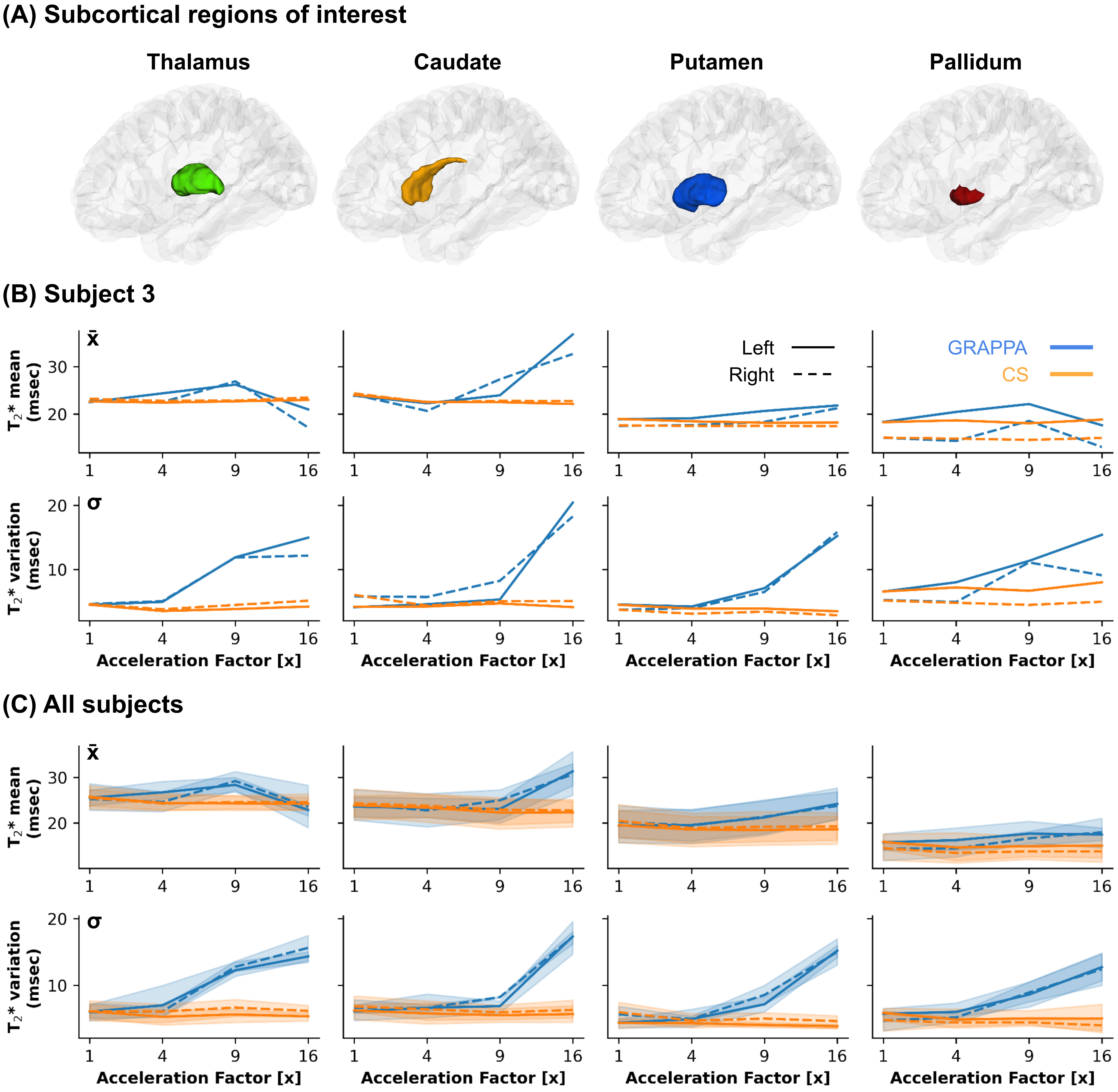
To evaluate the reconstructions, we used the NMSE and Pearson’s correlation coefficient for quantitative analysis as in4, and qualitatively by means of visual inspection. To evaluate T2* maps, we used the thalamic, caudate, putamen, and pallidum FreeSurfer labels to compare mean (x̄) and standard deviation (σ) for each subject at the different acceleration factors with the fully sampled reference. For region-wise analyses of the cortical data, we used the Glasser atlas13 to parcellate the cortical maps.
Results
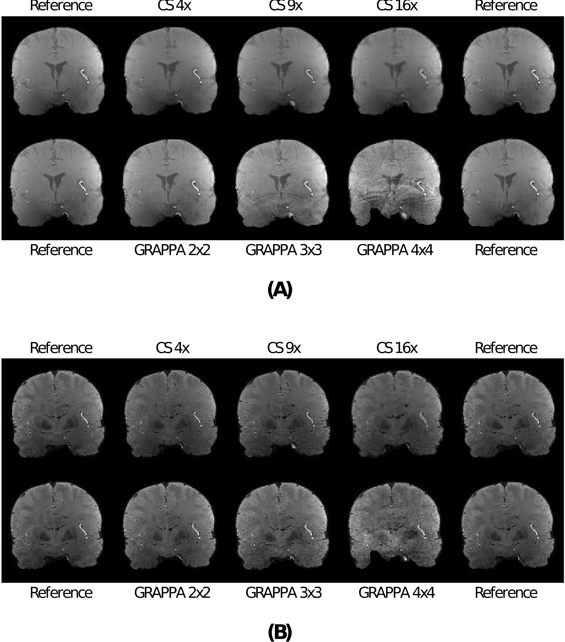
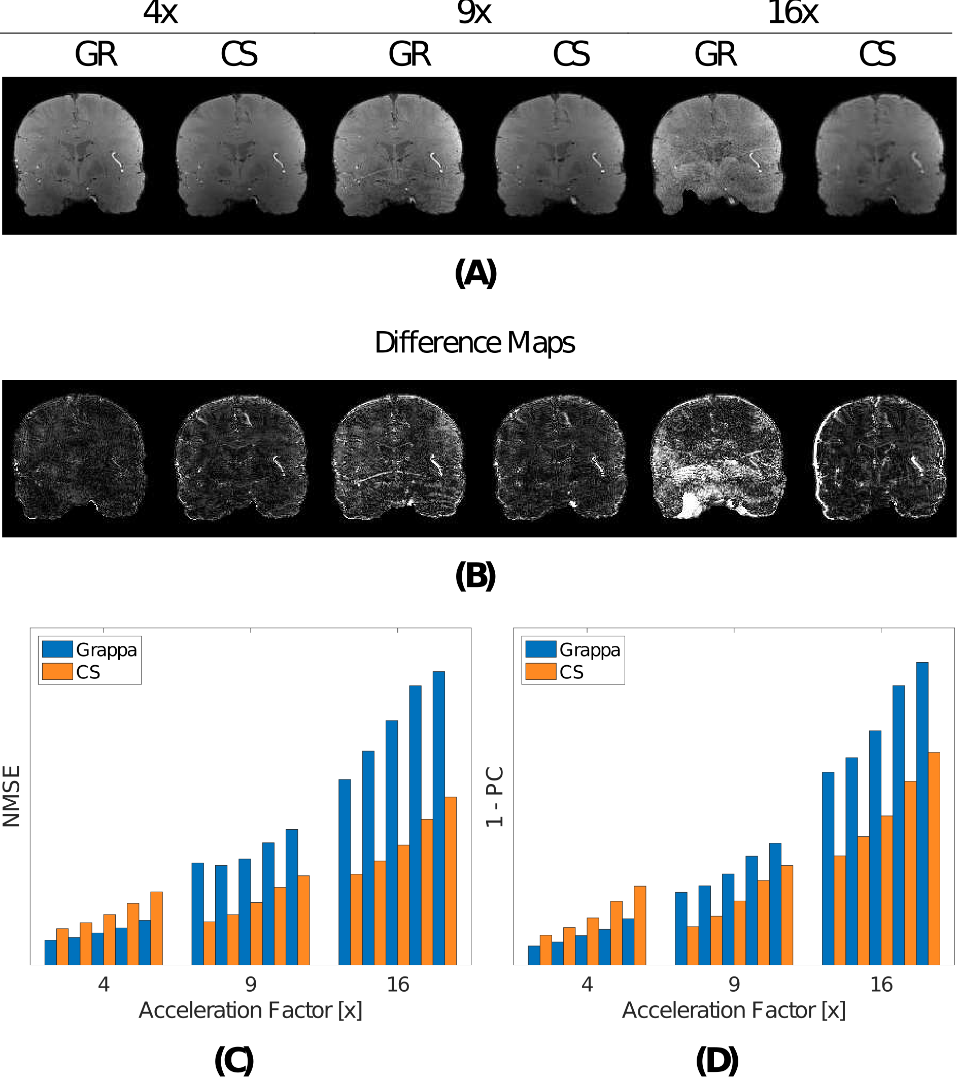
Figures 1 and 2 show the MRI magnitude images obtained using GRAPPA- and CS-based reconstructions. GRAPPA at 16x is corrupted by aliasing or diminished noise cancellation. On the other hand, CS at 16x introduces blurring but preserves structural content and coherence along all echoes. Additionally, in Figure 2 panels (C) and (D) reveal that both error indices increase with each new echo, and that the error from GRAPPA starts to be higher than for CS at 9x (and onwards).Figure 3 shows the subcortical T2* from the reconstructions. While average subcortical T2* appears relatively stable across acceleration factors for both reconstruction methods, its variability increases sharply for GRAPPA at 16x. This effect is observed across all subjects.
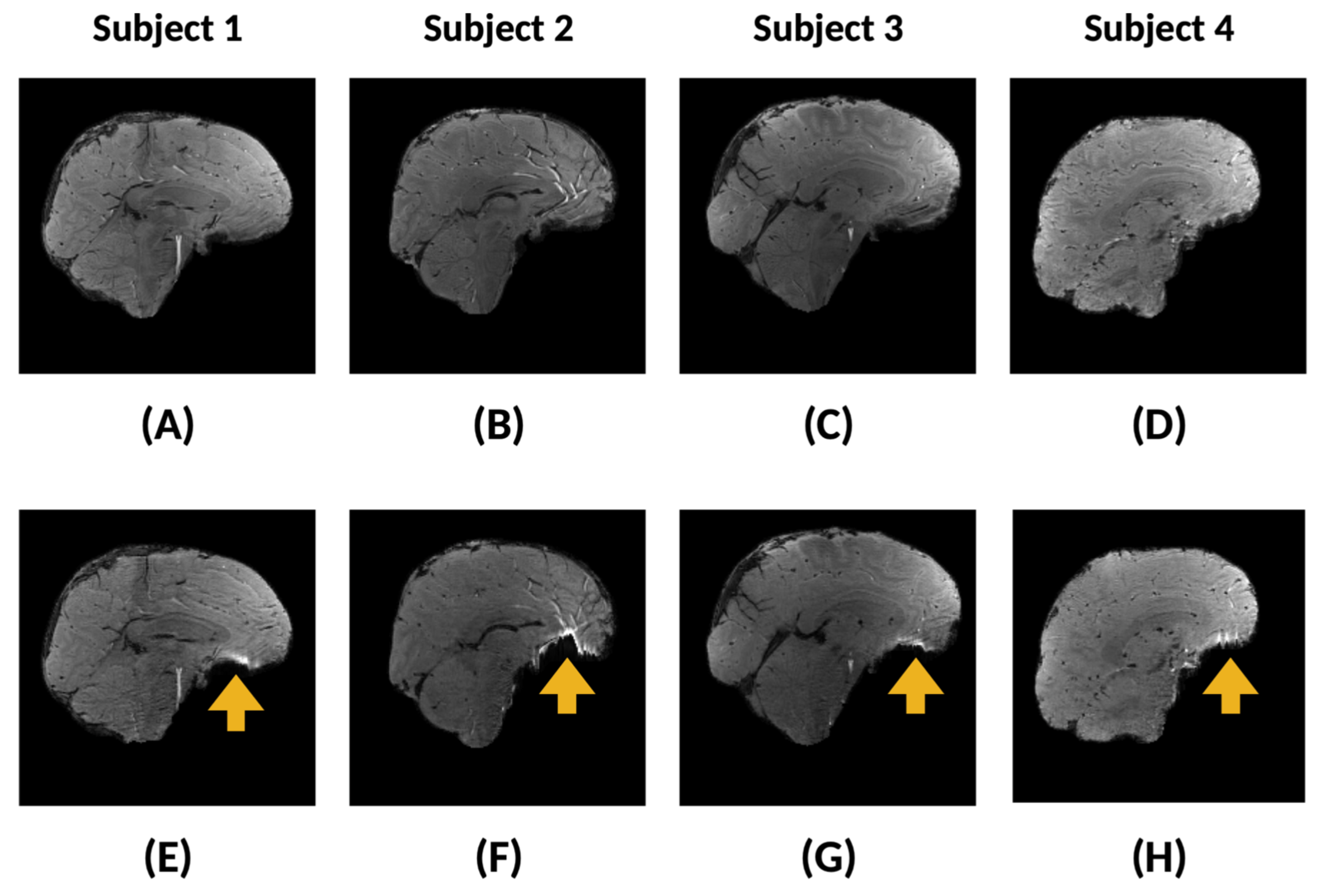
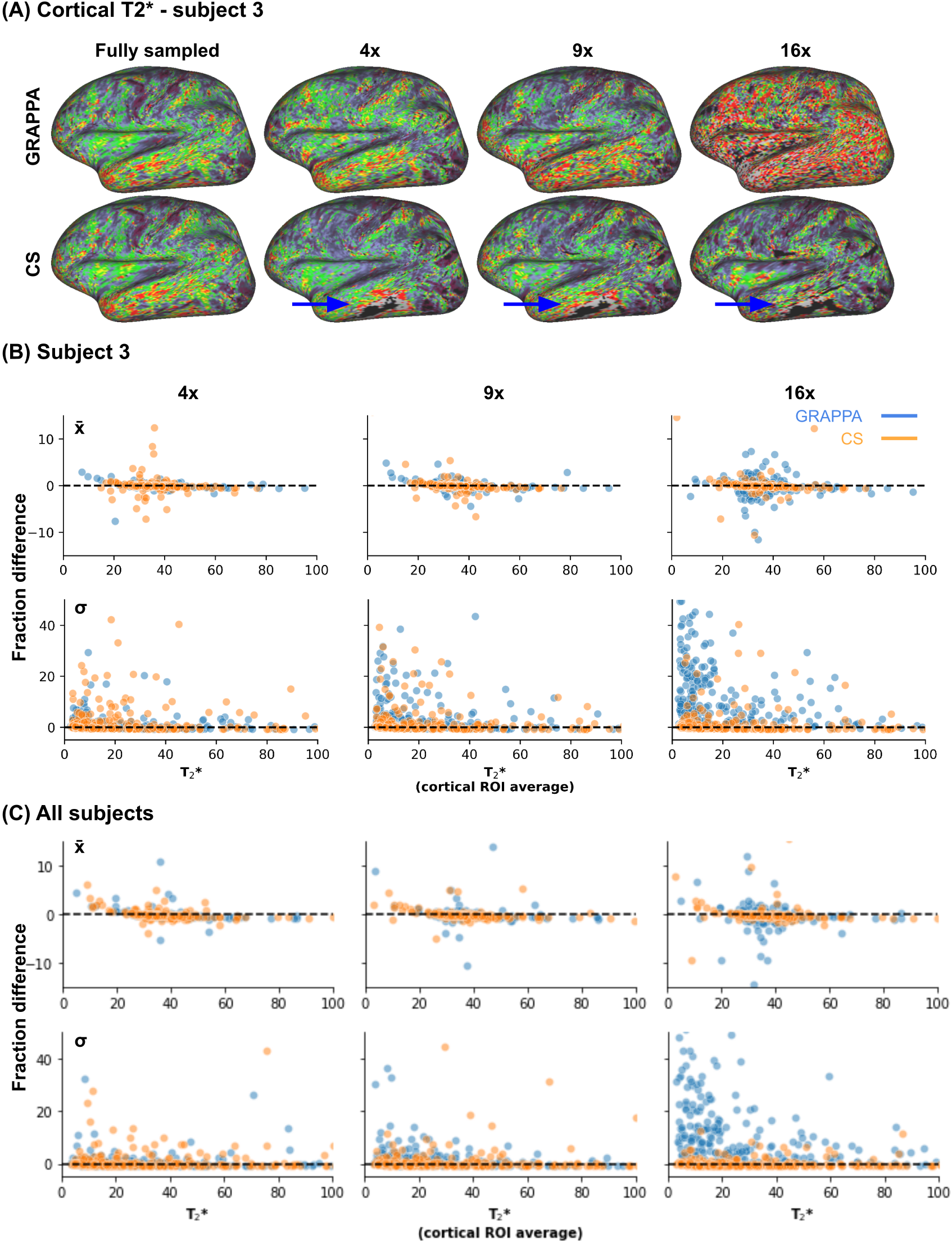
Figure 4 shows the inter-subject analysis on the sagittal plane. As depicted, geometrical distortions are detected in some parts of the cortex. These predominantly arise near air-tissue interfaces and increasing the spatial resolution could mitigate their effect14. Finally, Figure 5 shows the cortical T2* maps. In line with the subcortical results, cortical T2* remains stable for CS but breaks down at 16x for GRAPPA. The black zone near the inferior temporal lobe (see blue arrow in panel A) is a consequence of the geometric distortions observed in Figure 4.
Conclusion
In this work we compared GRAPPA and a novel CS-based reconstruction with automatic selection of the regularization weighting with up to 16-fold accelerated ME-GRE acquisitions. Results indicate a clear barrier that GRAPPA cannot exceed even with 32 receiving coils whereas CS-based reconstruction shows promising results to surpass that limit. These results could open the avenue for ultra-fast acquisitions for critically time-constrained MRI. However, current results also show some caveats (e.g., the geometric distortions) that need to be addressed in future work.Acknowledgements
Authors would like to thank Mr. Trevor Szkeres for assistance with data acquisition. This project was supported by a Canadian Institutes of Health Research (CIHR) grant FRN 148453 and NSERC Discovery grant to R.S.M.; and BrainsCAN, the Canada First Research Excellence Fund award to Western University. R.A.M.H. was supported by a BrainsCAN postdoctoral fellowship for this work. A.R.K was supported by a Canada Research Chairs award. Computational resources were provided by Compute Canada and a Canada Foundation for Innovation (CFI) John R. Evans Leaders Fund project 37427.References
1. Candes, E. J. & Wakin, M. B. An Introduction To Compressive Sampling. Ieee Signal Proc Mag 25, 21–30 (2008).
2. Donoho, D. L. Compressed Sensing. Ieee T Inform Theory 52, 1289–1306 (2006).
3. Lustig, M., Donoho, D. & Pauly, J. M. Sparse MRI: The application of compressed sensing for rapid MR imaging. Magnet Reson Med 58, 1182–1195 (2007).
4. Varela‐Mattatall, G., Baron, C. A. & Menon, R. S. Automatic determination of the regularization weighting for wavelet‐based compressed sensing MRI reconstructions. Magnet Reson Med 86, 1403–1419 (2021).
5. Gilbert, K. M. et al. Radiofrequency coil for routine ultra‐high‐field imaging with an unobstructed visual field. Nmr Biomed 34, e4457 (2021).
6. Ong, F., Cheng, J. Y. & Lustig, M. General phase regularized reconstruction using phase cycling. Magnet Reson Med80, 112–125 (2018).
7. Uecker, M. et al. ESPIRiT—an eigenvalue approach to autocalibrating parallel MRI: Where SENSE meets GRAPPA. Magnet Reson Med 71, 990–1001 (2014).
8. Marques, J. P. et al. MP2RAGE, a self bias-field corrected sequence for improved segmentation and T1-mapping at high field. Neuroimage 49, 1271–1281 (2010).
9. Smith, S. M. Fast robust automated brain extraction. Hum Brain Mapp 17, 143–155 (2002).
10. Wood, T. C. QUIT: QUantitative Imaging Tools. J Open Source Softw 3, 656 (2018).
11. Marcus, D. S. et al. Human Connectome Project informatics: Quality control, database services, and data visualization. Neuroimage 80, 202–219 (2013).
12. Haast, R. A. M. et al. Effects of MP2RAGE B1 + sensitivity on inter-site T1 reproducibility and hippocampal morphometry at 7T. Neuroimage 224, 117373 (2021).
13. Glasser, M. F. et al. A multi-modal parcellation of human cerebral cortex. Nature 536, 171–178 (2016).
14. Cohen-Adad, J. What can we learn from T2* maps of the cortex? Neuroimage 93, 189–200 (2014).
Figures