Introduction

When performing magnetic resonance spectroscopy of hydrogen, the abundant water present in the body can be used to determine the sensitivity maps. When imaging X-nuclei with custom coils, though, there is no sensitivity to water. In these situations, the sensitivity must be determined using the X-nuclei themselves. When sensing external contrast agents (e.g. imaging of phosphorus or hyperpolarized $$$^{13}C$$$), their lack of abundance presents precludes a high SNR measurement in every voxel.

For these applications, a common approach is the RefPeak method [1]. This method uses a single frequency to estimate the sensitivity maps, which yields a noisy result. It neglects to take full advantage of all of the information present in the received spectrum. In this work, we present a least-squares method that takes advantage of the multiple measurements made in all frequency bins.

Methods

Let $$$v^{(c)}$$$ denote the spectrum emitted by the isochromat of a given voxel received by the $$$c^{\text{th}}$$$ coil. Let $$$\rho\in\mathbb{C}^C$$$ denote a vector of coil sensitivity values for all coils at the location of the same voxel. The coil sensitivity values are those that satisfy the following for each frequency bin $$$\lambda$$$ [2,3]:
\begin{equation} \rho_c = \frac{ v^{(c)}_\lambda }{ \sqrt{ \sum_{\gamma=1}^C \left( v^{(\gamma)}_\lambda \right)^2 } } \hspace{1em} \Leftrightarrow \hspace{1em} v^{(c)}_\lambda=\rho_c\,\sqrt{\sum_{\gamma=1}^C \left( v^{(\gamma)}_\lambda \right)^2 }.\end{equation}
The RefPeak method determined $$$\rho_c$$$ using the value in the spectrum with the largest magnitude: $$$\rho_c = v^{(c)}_{\lambda_{\text{max}}} / \sqrt{ \sum_{\gamma=1}^C \left( v^{(\gamma)}_{\lambda_{\text{max}}} \right)^2 }$$$. Since $$$\rho_c$$$ is the same for all frequency bins, the equations above form a system of linear system of equations with a single scalar unknown, as follows:
\begin{equation}\begin{bmatrix}\sqrt{ \sum_{\gamma=1}^C \left( v^{(\gamma)}_1 \right)^2 } \\ \sqrt{ \sum_{\gamma=1}^C \left( v^{(\gamma)}_2 \right)^2 }\\ \vdots\\ \sqrt{ \sum_{\gamma=1}^C \left( v^{(\gamma)}_N \right)^2 } \end{bmatrix} \rho_c = \begin{bmatrix}v^{(c)}_1 \\ v^{(c)}_2 \\ \vdots \\ v^{(c)}_N\end{bmatrix}\hspace{1em} \Rightarrow\hspace{1em}\rho_c^{\star} = \begin{bmatrix}\sqrt{ \sum_{\gamma=1}^C\left( v^{(\gamma)}_1 \right)^2 }\\ \sqrt{ \sum_{\gamma=1}^C\left( v^{(\gamma)}_2 \right)^2 }\\ \vdots\\ \sqrt{ \sum_{\gamma=1}^C\left( v^{(\gamma)}_N \right)^2 }\end{bmatrix}^\dagger \begin{bmatrix}v^{(c)}_1\\ v^{(c)}_2\\ \vdots\\ v^{(c)}_N\end{bmatrix}, \label{eq:lsSensitivity}\end{equation}
where there are $$$N$$$ bins in the spectrum, and $$$^\dagger$$$ represents the pseudoinverse. This linear system can be solved numerically using the QR decomposition [4]. Notably, this technique can be used whenever multiple measurements are attained of a given voxel with the same sensitivity. For example, with dynamic data, one makes multiple images of the same subject with contrast that varies over time. For this application, the variable $$$\lambda$$$ can index time, and the sensitivity of the voxel can be estimated by solving the above matrix equation where there is one element in each of the vectors for each point in time.

Once the sensitivity maps are estimated, a single image can be reconstructed using the method of Roemer [2]. Alternatively, one can perform a model based reconstruction with a non-trivial prior [5]. We present results using both techniques below. For the model based reconstruction, we demonstrate results from solving the following optimization problem with Tikhonov regularization:
\begin{equation}\underset{x}{\text{minimize}}\hspace{0.5em}\left\|D\,F\,x-b\right\|_2^2+\mu\,\|x\|_2^2, \label{eq:modelBasedRecon}\end{equation}
where $$$x$$$ is the reconstructed image, $$$F$$$ is the Fourier transform, $$$D$$$ is the downsampling matrix indicating which samples were acquired, and $$$x$$$ represents the image.

Results

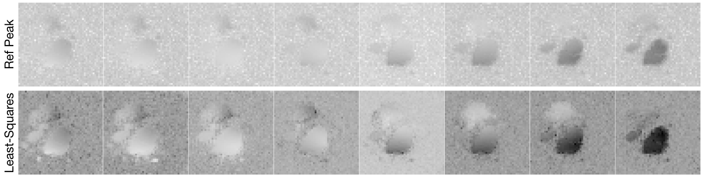
We present results from two experiments: 1) a dynamic acquisition of the heart after an injection of hyperpolarized [1-$$$^{13}C$$$] where spectral-spatial pulses were used to individually excite and acquire images of pyruvate, lactate, and bicarbonate, and 2) an Echo Planar Spectroscopic Imaging (EPSI) of the brain after an injection of hyperpolarized [1-$$$^{13}C$$$] pyruvate.

Figure-1 shows the sensitivity maps of the heart generated from images of hyperpolarized [1-$$$^{13}C$$$] using both the RefPeak method and the new least-squares method. The data from all times and all three metabolites were used to estimate the sensitivity maps. All sensitivity maps are displayed on the same dynamic scale. The sensitivity maps generated from the least-squares approach present significantly reduced noise in areas of the images absent of any sample. Additionally, the sensitivities estimated in the superior regions of the image are more pronounced.

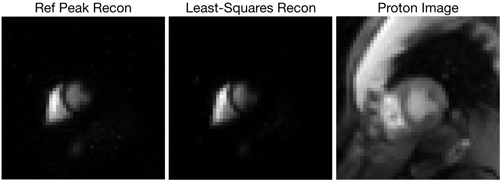
Figure-2 shows a slice of the heart where individual coil images have been combined using the method of Roemer [2] with sensitivity maps generated from the RefPeak and least-squares method; these images are placed beside a corresponding proton image. Note that the least-squares image better localizes the signal of pyruvate in the left and right ventricles.

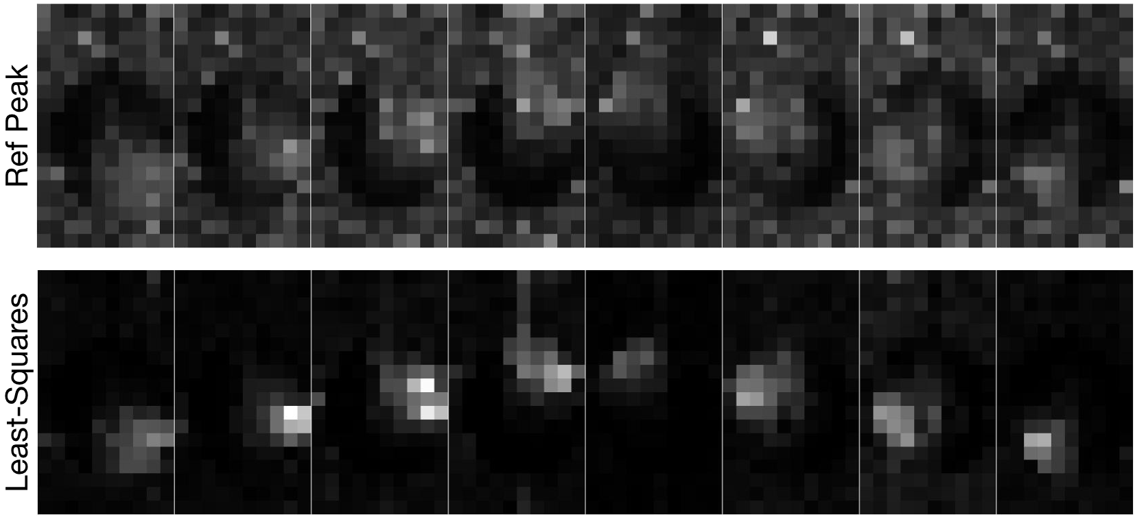
Figure-3 shows the sensitivity maps estimated using the RefPeak method and the least-squares method for the EPSI brain data. Note that the least-squares sensitivity maps show far less noise than the maps generated with the RefPeak method. As before, note the reduced noise in the regions absent of tissue.

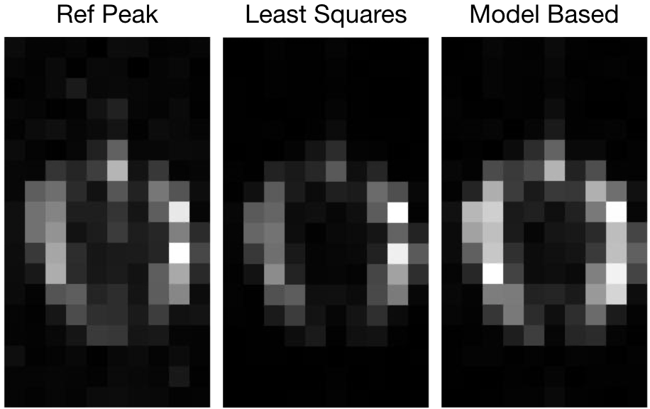
Figure-4 shows the area-under-the-curve reconstructions of the brain using the RefPeak and least-squares sensitivity maps with the Roemer method. Additionally, the existence of accurate sensitivity maps permits the reconstruction with a model based approach; figure-4 also shows the model based reconstruction. The RefPeak reconstruction presents the highest intensity outside of the skull, which is undesired. Horizontal symmetry, which is desired, is greatest in the model-based reconstruction.

Conclusion

In this work, we present a least-squares method for estimating the sensitivity of a voxel when imaging X-nuclei. We show results with cardiac data and the brain. And we show that the existence of accurate sensitivity maps permits reconstruction using a model based algorithm when imaging X-nuclei.

References

[1] Emma L Hall, Mary C Stephenson, Darren Price, and Peter G Morris. Methodology for improved detectionof low concentration metabolites in mrs: optimised combination of signals from multi-element coil arrays. Neuroimage, 86:35–42, 2014.
[2] Peter B Roemer, William A Edelstein, Cecil E Hayes, Steven P Souza, and Otward M Mueller. The NMR phased array. Magnetic Resonance in Medicine, 16(2):192–225, 1990.
[3] Erik G Larsson, Deniz Erdogmus, Rui Yan, Jose C Principe, and Jeffrey R Fitzsimmons. SNR-optimality of sum-of-squares reconstruction for phased-array magnetic resonance imaging. Journal of MagneticResonance, 163(1):121–123, 2003.3
[4] Lloyd N Trefethen and David Bau III. Numerical linear algebra, volume 50. Society of Industrial andApplied Mathematicians, 1997.
[5] Jeffrey A Fessler. Model-based image reconstruction for MRI. IEEE signal processing magazine, 27(4):81–89, 2010.