2437
Training a tunable, spatially-adaptive denoiser without clean targets1Pattern Recognition Lab, Friedrich-Alexander-University Erlangen-Nuremberg, Erlangen, Germany, 2MR Application Predevelopment, Siemens Healthcare GmbH, Erlangen, Germany
Synopsis
Accelerating MRI is intrinsically limited by the thermal noise from the imaged object. In this work we aim to optimize MR image denoising using an unsupervised deep learning-based method. Stein's unbiased risk estimator and spatially resolved noise maps indicating the standard deviation of the noise for every pixel were incorporated into the training process. It was shown that this approach can achieve results that are equal or superior to those of state-of-the-art supervised and unsupervised methods. Furthermore, we show how to control the tradeoff between denoising and image sharpness by using a model conditioned on the noise map.
Introduction
In MRI, sufficient signal-to-noise-ratio is a key requirement for achieving diagnostic image quality. Since the acquired noise for clinical scanners is dominated by thermal noise from the imaged object, there is a natural barrier for noise reduction. The noise distribution can be modelled as Gaussian and may be determined by a noise adjustment scan. With conventional image reconstruction being almost linear, the spatially-variant noise distribution in the final images can be obtained by propagation through the reconstruction algorithm.In recent years, deep learning (DL)-based methods have been successfully employed to remove noise from images post acquisition. Supervised DL approaches require pairs of noisy and noise-free images for training, but the acquisition of noise-free images is usually difficult or even impossible in the context of medical imaging. For such cases, unsupervised learning methods can be applied, which do not require noise-free target images for training. A promising unsupervised approach is the use of Stein's unbiased risk estimator (SURE)1 as loss function during training, which approximates the mean squared error (MSE) between denoised and clean images by incorporating the variance of the underlying noise distribution.
Putting the ability to obtain quantitative noise maps and previous work on the removal of univariate Gaussian noise together, we extended the SURE approach to MR imaging, focusing on conventional 2D TSE acquisitions.
Methods
To properly address the spatially-variant noise enhancement in complex-valued MR images, the SURE-based approach proposed by Metzler et al.2 was adapted accordingly. Instead of a univariate model, the resulting formulation incorporates a noise map indicating the standard deviation of the noise for every pixel.The noisy measurement vector $$$\bf{y}\in\mathbb{R}^{D}$$$ is assumed to follow a multivariate Gaussian distribution with clean image $$$\bf{x}\in\mathbb{R}^{D}$$$ as mean and covariance matrix $$$\boldsymbol{\Sigma}$$$ coming from the additive noise $$$\boldsymbol{\eta}\sim\mathcal{N}(0,\boldsymbol{\Sigma})$$$. We assume noise is independently distributed for each pixel. Therefore, $$$\boldsymbol{\Sigma}$$$ is a diagonal matrix with entries $$$\Sigma_{ii}=\sigma_i^2$$$, where $$$\sigma_i$$$ are the components of the noise map $$$\boldsymbol{\sigma}\in{\mathbb{R}}^{D}$$$. Suppose $$$\boldsymbol{f}(\boldsymbol{y})$$$ is an estimator of the unknown ground truth $$$\boldsymbol{x}$$$ from $$$\boldsymbol{y}$$$ defined as $$$\boldsymbol{f}(\boldsymbol{y})=\boldsymbol{y}+\boldsymbol{g}(\boldsymbol{y})$$$, where $$$\boldsymbol{g}$$$ is a weakly differentiable function, then the MSE can be expressed as the expectation of SURE with respect to $$$\boldsymbol{x}$$$:
$$\text{MSE}(\boldsymbol{f})=\text{E}_{\boldsymbol{x}}\Big\{\,\Vert\boldsymbol{f}(\boldsymbol{y})-\boldsymbol{y}\Vert^2-\sum\nolimits_i^D\sigma_i^2+2\text{div}_{\boldsymbol{y}}\big(\,\boldsymbol{\sigma^2}\odot\boldsymbol{f}(\boldsymbol{y})\big)\,\Big\}\,,$$
where $$$\text{div}_{\boldsymbol{y}}$$$ is the divergence with respect to $$$\boldsymbol{y}$$$ defined as:
$$\text{div}_{\boldsymbol{y}}\big(\,\boldsymbol{\sigma^2}\odot\boldsymbol{f}(\boldsymbol{y})\big)\,\approx\boldsymbol{b}^T\bigg(\,\boldsymbol{\sigma^2}\odot\Big(\,\frac{\boldsymbol{f}(\boldsymbol{y}+\epsilon\boldsymbol{b})-\boldsymbol{f}(\boldsymbol{y})}{\epsilon}\Big)\,\bigg)\,.$$
Here $$$\odot$$$ denotes element-wise multiplication, $$$\bf{b}\in\mathbb{R}^{D}$$$ is defined as a zero-mean i.i.d. random vector with unit variance and $$$\epsilon$$$ is a small value close to zero, for instance $$$\epsilon=\text{max}(\bf{y})\cdot10^{-3}$$$.
The noise map was computed by propagating the original univariate noise distribution through all steps of the image reconstruction pipeline3,4, as illustrated in Figure 1.
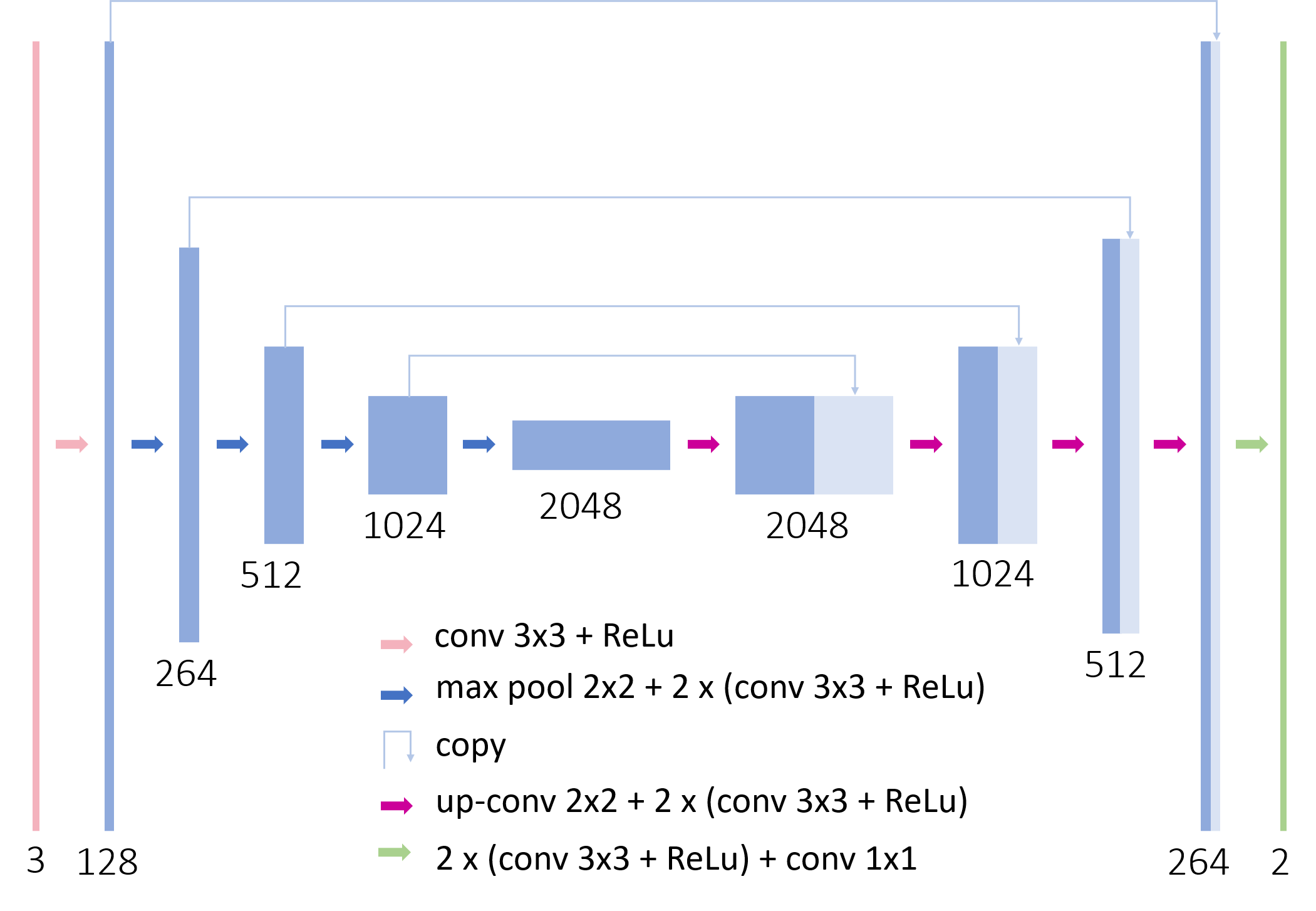
The unsupervised SURE-based training approach was compared with two supervised loss functions MSE and structural similarity index measure (SSIM) as well as the unsupervised method Noise2Void5. To enable supervised training, images obtained with 1.5 and 3 T scanners (MAGNETOM Vida, Lumina, Altea and Sola, Siemens Healthcare, Erlangen, Germany) were used as ground truth. The images were acquired from volunteers in various body regions using typical acquisition protocols for the respective clinically relevant contrasts. The noisy network input for both supervised and unsupervised methods was then obtained by adding synthetic noise to the images based on the corresponding noise maps. The U-Net6-based architecture in Figure 2 was implemented in PyTorch and trained with 8,201 images. The denoising results were quantitatively evaluated by calculating MSE, SSIM and peak signal-to-noise-ratio (PSNR) between the denoised images and the original images for 2,602 test samples.
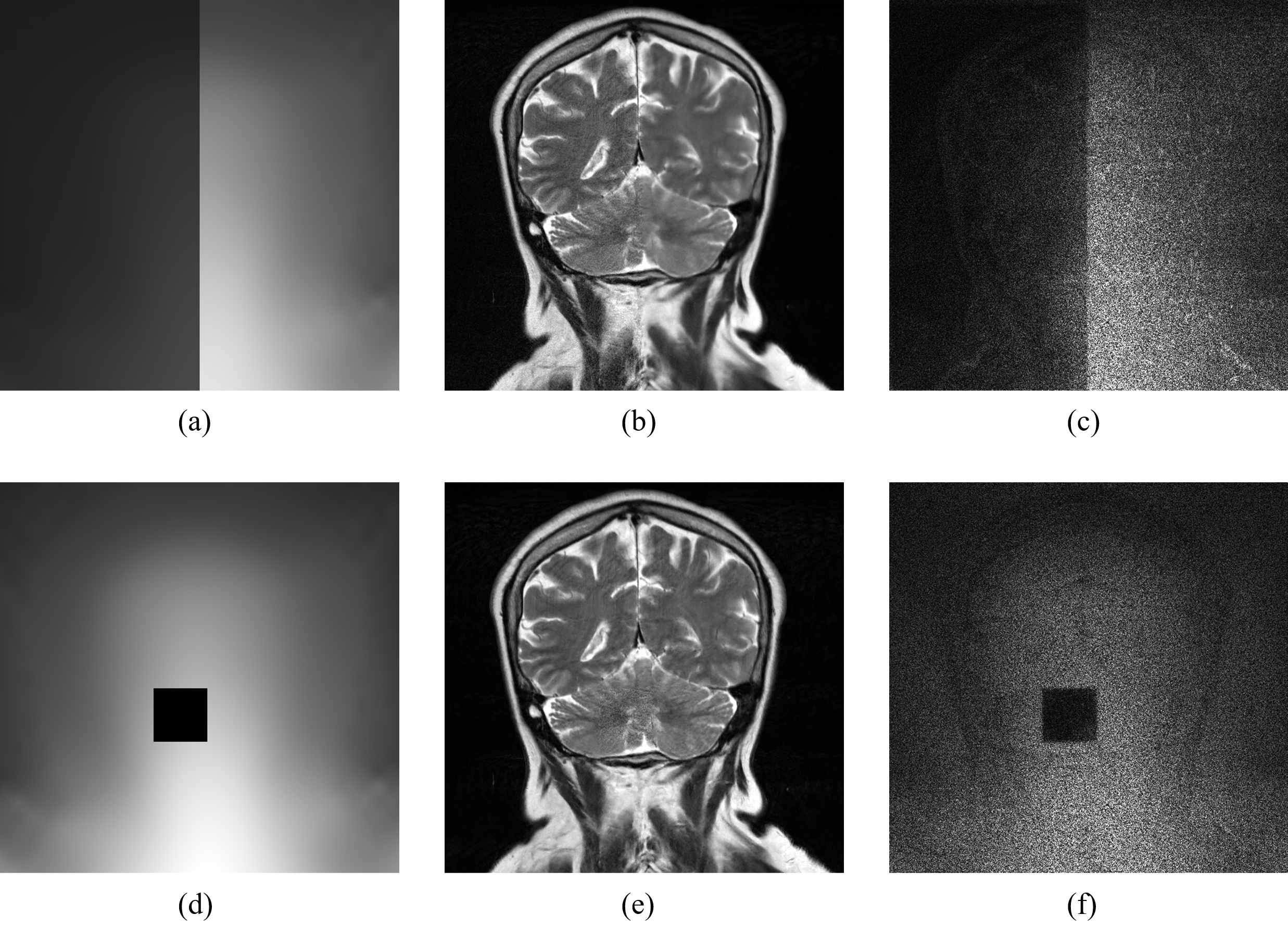
To be able to regulate the denoiser in a fine-grained manner, the noise maps were fed into the network as an additional input channel, resembling the approach presented by Zhang et al.7. To analyze their influence during inference, noise maps of exemplary images were manipulated in several ways.
Results
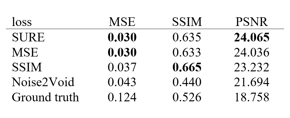
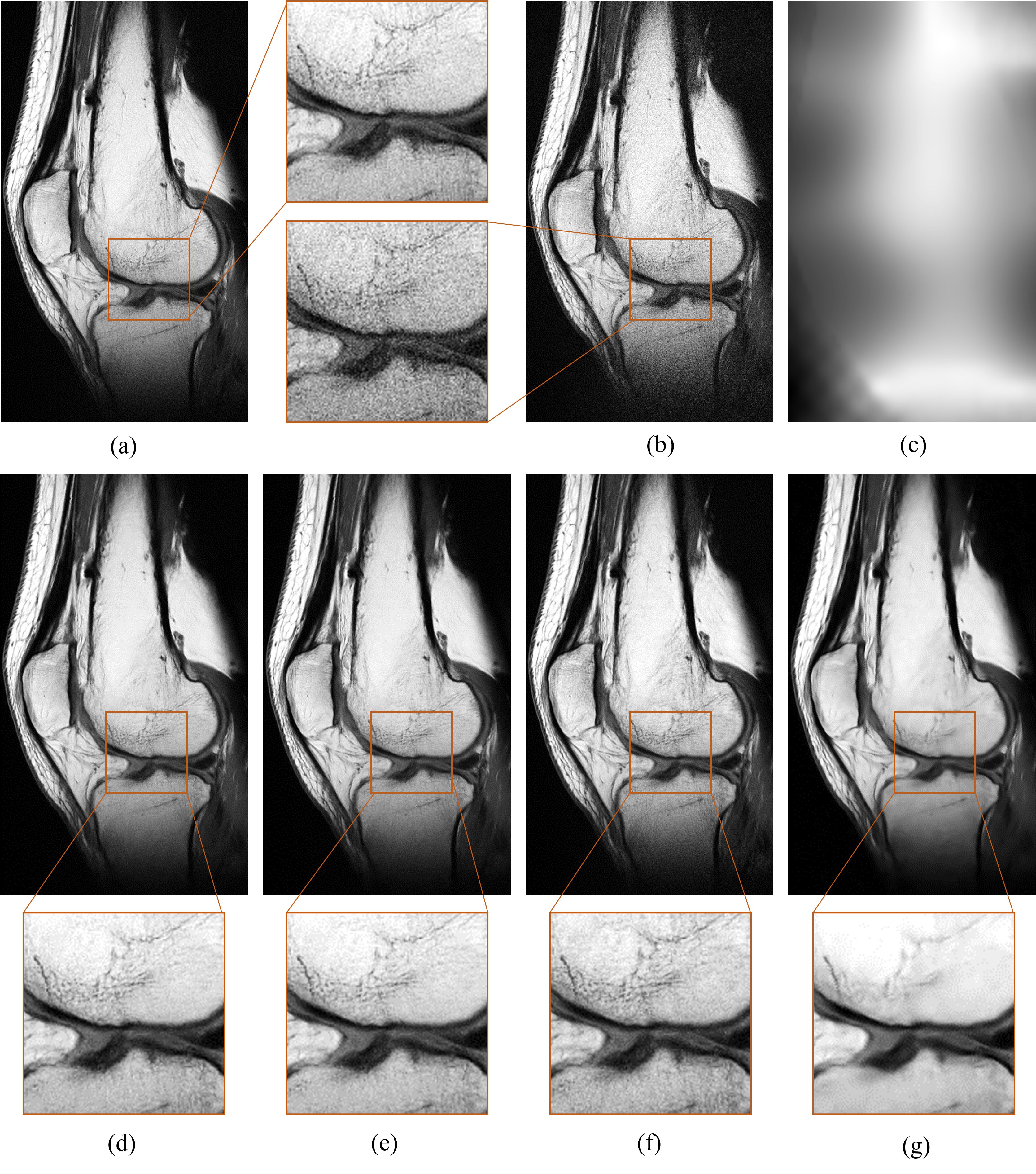
A comparison of the different training methods is presented in Table 1. Although the network trained with SURE loss did not require noise-free target images, the results were at least equivalent to the network trained in a supervised manner with MSE loss and clearly outperformed the Noise2Void-based network. An example of a visual comparison is depicted in Figure 3. The images that were denoised with networks based on SURE and MSE appear smoother and contain even less noise than the original image. For the network trained with SSIM, the result image appears slightly sharper because it displays additional noise and more prominent edges. In contrast, the result obtained with Noise2Void shows significant loss in resolution. Additionally, it was found that the incorporation of the noise map during inference allows to customize the level of denoising by scaling the noise map. Figure 4 illustrates the local adaptation of denoising strength.Discussion
We demonstrated that the proposed unsupervised SURE-based method can compete with supervised approaches by incorporating supplementary information about the local noise level, which makes it particularly interesting for cases where no ground-truth data is available. The integration of the noise map as a third input channel brings a significant advantage by allowing the denoising level to be adjusted as desired.Conclusion
Our denoising method might be beneficial for low-field image denoising or to shorten scan times by accepting higher noise levels through, e.g., higher bandwidth imaging or fewer averages.Acknowledgements
No acknowledgement found.References
- Stein C. Estimation of the mean of a multivariate normal distribution. The Annals of Statistics 1981; 9(6):1135–1151.
- Metzler C et al. Unsupervised learning with Stein’s unbiased risk estimator. arXiv preprint arXiv:1805.10531, 2018.
- Breuer F et al. General formulation for quantitative g-factor calculation in GRAPPA reconstructions. Magnetic Resonance in Medicine 2009; 62(3):739-746.
- Belaroussi B et al. Intensity non-uniformity correction in MRI: existing methods and their validation. Medical Image Analysis 2006; 10(2):234-246.
- Krull A et al. Noise2Void-learning denoising from single noisy images. In Proceedings of the IEEE/CVF Conference on Computer Vision and Pattern Recognition 2019; 2129–2137.
- Ronneberger O et al. U-Net: Convolutional networks for biomedical image segmentation. In International Conference on Medical Image Computing and Computer-Assisted Intervention 2015; 234–241.
- Zhang K et al. FFDNet: Toward a fast and flexible solution for CNN-based image denoising. IEEE Transactions on Image Processing 2018; 27(9):4608–4622.
Figures
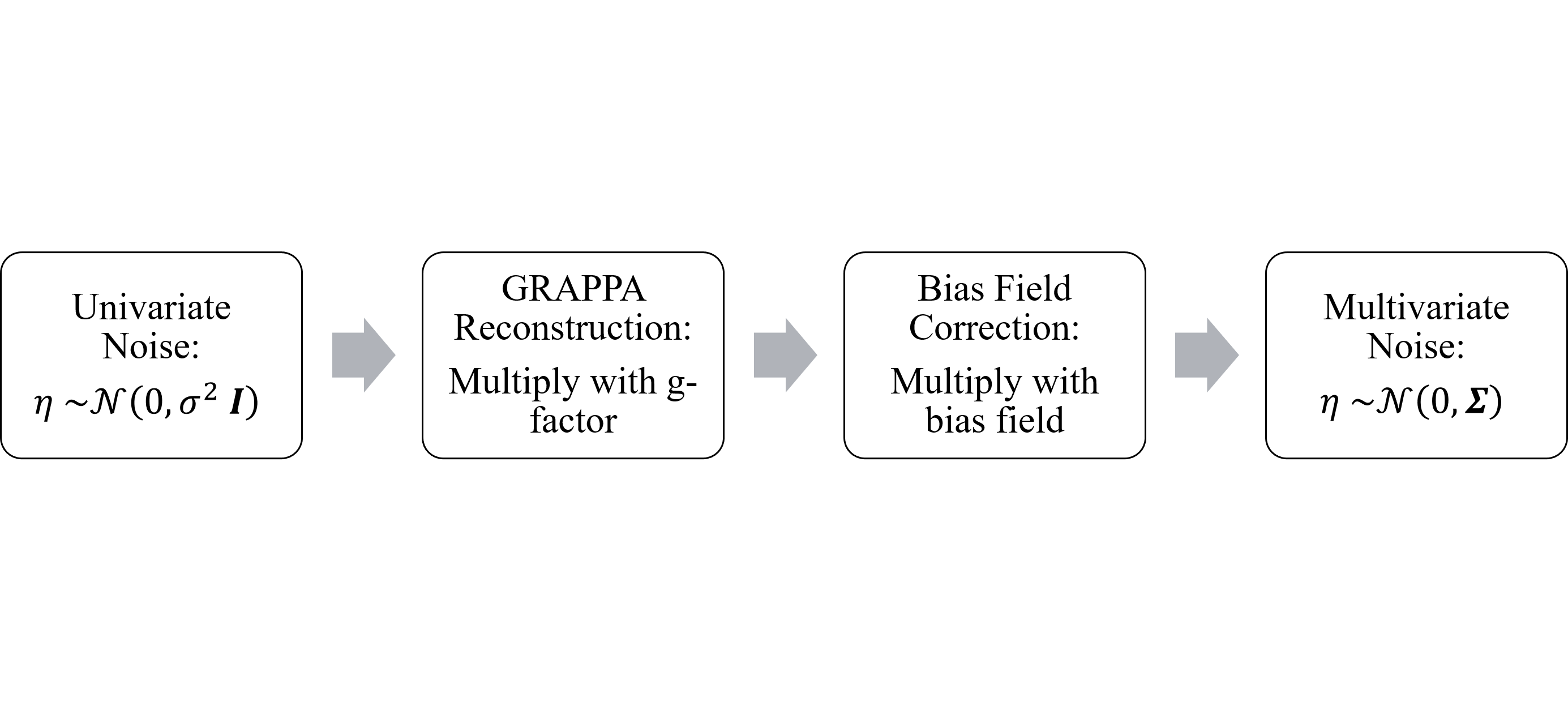
Figure 1: The process for calculating the noise maps. The initially univariate thermal noise distribution, which can be determined by a noise adjustment scan, is propagated through the image reconstruction pipeline, resulting in a multivariate Gaussian distribution. Σ can be interpreted as a diagonal matrix with entries Σii = σi2, where σi are the components of the noise map σ.