2435
Open-source model-based reconstruction in Julia: A pipeline for spiral diffusion imaging1Techna Institute, University Health Network, Toronto, ON, Canada, 2UBC MRI Research Center, University of British Columbia, Vancouver, BC, Canada, 3Techna Institute & Koerner Scientist in MR Imaging, University Health Network, Toronto, ON, Canada, 4Biomedical Engineering, Center for Neuroscience Imaging Research, Institute for Basic Science, Sungkyunkwan University, Suwon, Korea, Republic of
Synopsis
We investigated the use of physically-motivated corrections for non-Cartesian imaging within a fast, open-source MR reconstruction framework written in the Julia programming language. Building on existing Julia libraries for MR image reconstruction, we developed a comprehensive, open-source pipeline for non-Cartesian image reconstruction including B0 inhomogeneity correction, gradient system characterization and eddy current correction. We demonstrated that spiral images can be reconstructed using this pipeline with high geometric accuracy in a fast, accessible and efficient manner on modest hardware.
Introduction
Image acquisition with non-Cartesian k-space trajectories permits time efficient MR imaging and improved image quality such as reduced distortions, allowing for both high temporal and spatial resolution. However, the sensitivity of such trajectories to system imperfections presents a significant barrier to robust and accurate image reconstruction.1 Effective strategies to correct these imperfections have been developed and were shown to be necessary for accurate spiral imaging reconstruction.2-7 However, widespread use of such strategies is hindered by development cost, the need for additional calibration scans and hardware, and the use of proprietary image reconstruction code.Further adoption of non-Cartesian sequences requires an accessible, hardware-independent framework for accounting system imperfections at the time of image reconstruction. The development of open-source, extensible MR image reconstruction frameworks (MRIReco.jl) capable of handling arbitrary trajectories and expanded signal models have made efficient and generalized non-Cartesian image reconstruction accessible.2,8 In the present work, we demonstrate a comprehensive, open-source pipeline for the reconstruction of images acquired using spiral k-space trajectories. The pipeline is built around MRIReco.jl and ISMRMRD, and incorporates B0 correction, correction for trajectory imperfections using the Gradient Impulse Response Function (GIRF), and eddy current compensation prior to reconstruction.8,9 We found Julia to be a robust language for MR imaging applications and assessed improvements to geometric fidelity of the reconstructed image achieved through incorporation of physically motivated corrections.
Methods
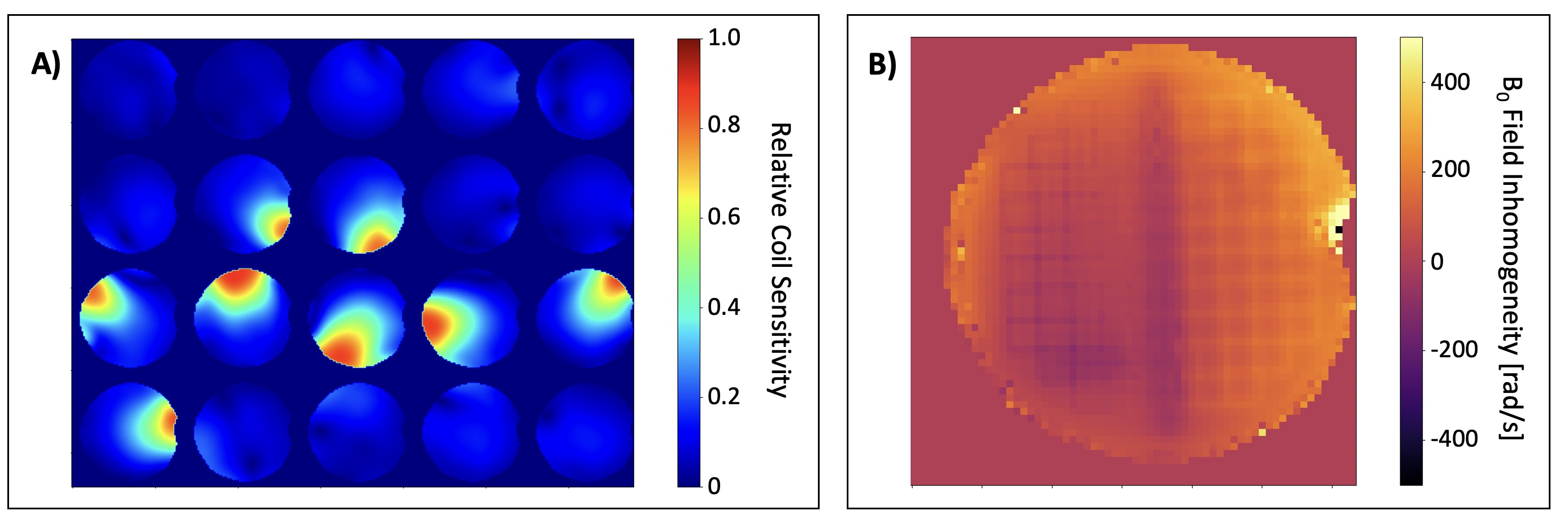
ImagingImage acquisition was performed on a Siemens Prisma 3T system, using a 4 interleave spiral trajectory (FOV 220mm/in-plane resolution 1.1mm) with uniform radial density and a readout duration of 31.54ms for each shot, time-optimal for the gradient.10 Nine transverse imaging slices (slice thickness = 3mm, slice gap 24mm) of the ACR geometric reference phantom were acquired, using a 20 channel head-neck coil. A dual-echo gradient echo scan (DE-GRE, TE1,2 = 4.92/7.42ms) of the ACR phantom was acquired with the same geometry, providing a reference for reconstruction accuracy and calibration data for B0 map and coil sensitivity estimation (Fig. 2).
Gradient System Characterization
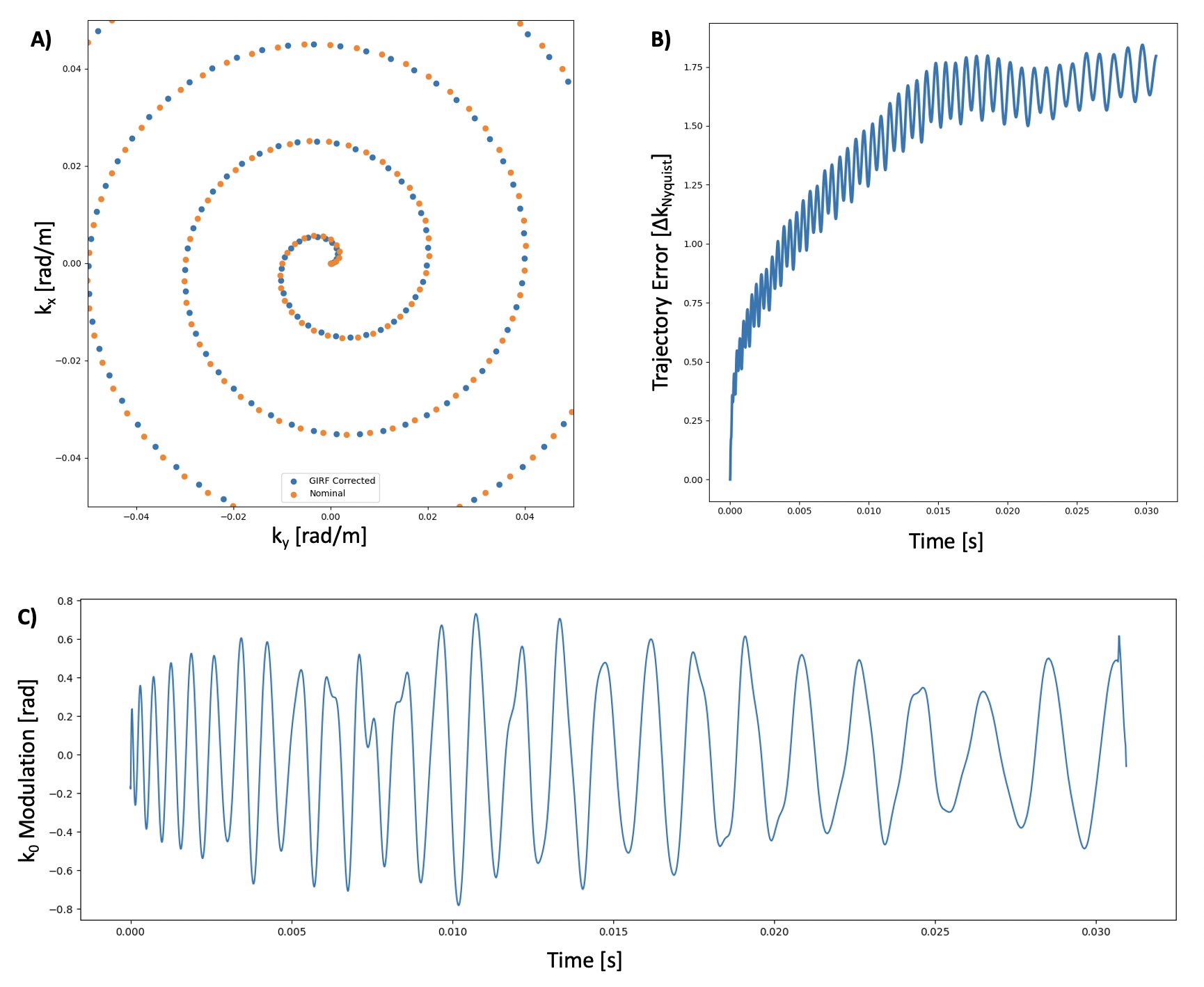
In a separate experiment, the MR gradient system performance was characterized by measurement of signal phase during gradient application, assuming a linear, time-invariant magnetic field response to input gradient waveforms.4 Gradient impulse response functions (GIRFs) were computed to first order, including the eddy current term k0.2,12,13 The corrected spiral trajectory was estimated via convolution with the GIRF.4
Image Reconstruction Pipeline and Quality Assessment
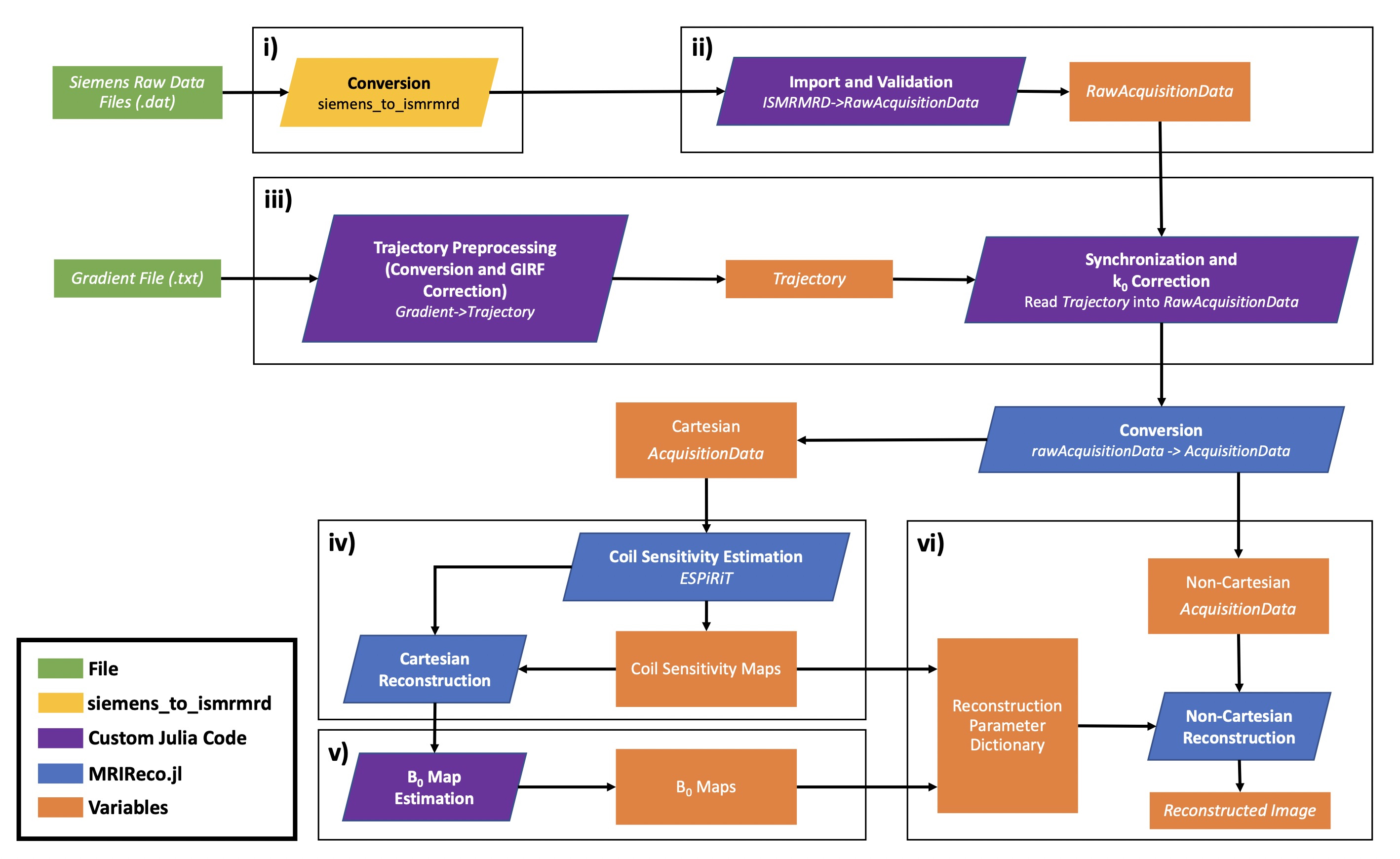
The end-to-end reconstruction pipeline from Siemens raw k-space data to spiral images is depicted in Figure 1, highlighting the inclusion of established open-source 3rd party tools (blue and yellow), as well as the custom modules developed in this work (purple).
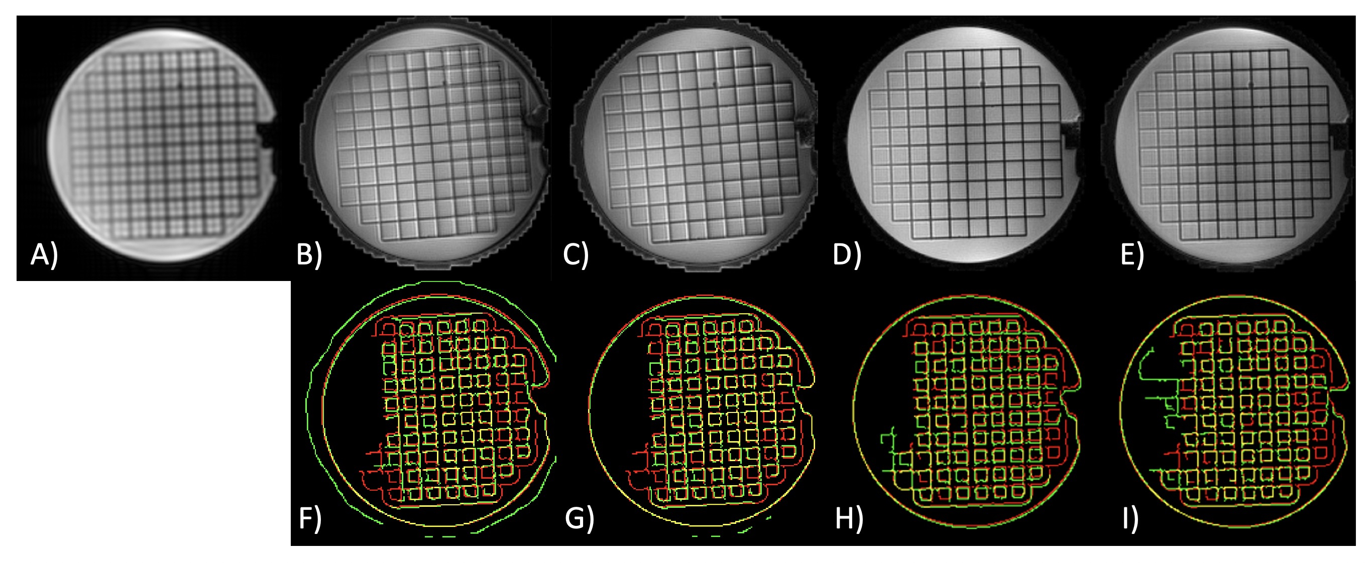
Geometric fidelity of reconstructed spiral images was assessed by comparison to the reference gradient-echo image and correspondence between image edges, using edge detection code written in Julia.
The impact of different pipeline modules on spiral reconstruction quality was evaluated by successive incorporation of the individual corrections:
- Uncorrected reconstruction: nominal spiral trajectory, no B0 correction
- Nominal spiral trajectory + B0 correction
- GIRF-predicted spiral trajectory + B0 correction
- GIRF-predicted k0 eddy current + GIRF-predicted spiral trajectory + B0 correction
Results
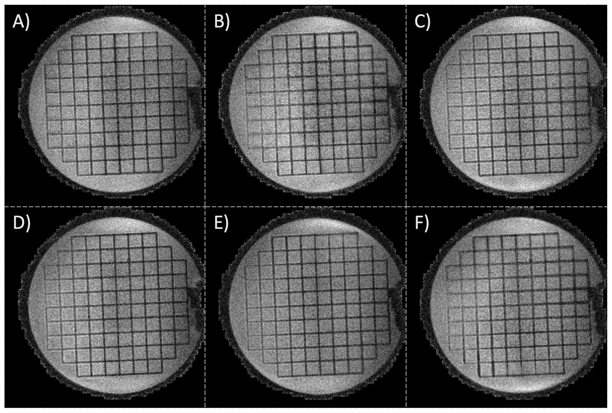
Measured B0 maps (Fig. 2B) show high homogeneity within the ACR phantom, with a maximum intra-slice variation of 130 Hz. The GIRF-predicted corrections to the spiral trajectory are small (Fig. 3A,B), at most 1.75x the Nyquist sampling interval. Despite these small imperfections, the reconstruction based on the nominal spiral trajectory without B0 correction exhibits severe blurring artifacts, image intensity modulations and geometric inaccuracies (Fig. 4B, 4F). Reconstruction with B0 correction significantly reduces blurring (Fig. 4C, 4G). Reconstruction with the corrected spiral trajectory obtained from GIRF prediction reduces geometric inaccuracy due to gradient delays (Fig. 4D, 4H). Finally, incorporation of GIRF-predicted k0 correction (Fig. 3C) leads to virtually artifact-free spiral image reconstructions with geometric congruency between GRE and spiral scans. (Fig. 4E, 4I).The versatility of the pipeline is shown in Fig. 5 for the reconstruction of b=1000 diffusion-weighted images. The corrections applied are effective even in the presence of diffusion-weighting gradients, with residual imperfections presumably due to higher-order effects.3
Reconstruction time with B0, GIRF and k0 correction was 19 seconds per slice when run on an Apple M1 MacBook Air.
Discussion
We demonstrated fast, high-quality spiral diffusion imaging enabled by a modular, open-source reconstruction pipeline written in Julia. The incorporation of GIRF and B0 correction was accommodated within Julia and was necessary for accurate spiral reconstruction, as previously shown.4,11-13 The computational efficiency of Julia and MRIReco.jl enable reasonably fast image reconstruction on modest hardware. In combination with the open and streaming-capable ISMRMRD format, real-time robust spiral image reconstruction can be realized.9 No additional hardware was needed to achieve high reconstruction quality, and the ISMRMRD file interface makes the framework vendor- and system-agnostic. The modularity of the presented pipeline lends itself to further development of the reconstruction framework to address remaining imperfections (Fig. 5).2,3To make such corrections easily accessible to the broader MR imaging community and add to the growing list of MR reconstruction tools available in Julia,8 this reconstruction pipeline will be available on GitHub and as a package within the Julia ecosystem (GIRFReco.jl).
Acknowledgements
All work was completed at the Brain-TO Lab in Toronto under the supervision of Dr. Kamil Uludag, Dr. Lars Kasper and Dr. Zhe (Tim) Wu.References
1. K. T. Block and J. Frahm, “Spiral imaging: A critical appraisal,” J. Magn. Reson. Imaging, vol. 21, no. 6, pp. 657–668, Jun. 2005, doi: 10.1002/jmri.20320.
2. B. J. Wilm, C. Barmet, M. Pavan, and K. P. Pruessmann, “Higher order reconstruction for MRI in the presence of spatiotemporal field perturbations: Higher Order Reconstruction for MRI,” Magn. Reson. Med., vol. 65, no. 6, pp. 1690–1701, Jun. 2011, doi: 10.1002/mrm.22767.
3. B. J. Wilm et al., “Diffusion MRI with concurrent magnetic field monitoring,” Magn. Reson. Med., vol. 74, no. 4, pp. 925–933, 2015, doi: 10.1002/mrm.25827.
4. S. J. Vannesjo et al., “Image reconstruction using a gradient impulse response model for trajectory prediction: GIRF-Based Image Reconstruction,” Magn. Reson. Med., vol. 76, no. 1, pp. 45–58, Jul. 2016, doi: 10.1002/mrm.25841.
5. S. J. Vannesjo et al., “Gradient system characterization by impulse response measurements with a dynamic field camera,” Magn. Reson. Med., vol. 69, no. 2, pp. 583–93, Feb. 2013, doi: 10.1002/mrm.24263.
6. A. K. Funai, J. A. Fessler, D. T. B. Yeo, V. T. Olafsson, and D. C. Noll, “Regularized Field Map Estimation in MRI,” IEEE Trans. Med. Imaging, vol. 27, no. 10, pp. 1484–1494, Oct. 2008, doi: 10.1109/TMI.2008.923956.
7. M. Uecker et al., “ESPIRiT-an eigenvalue approach to autocalibrating parallel MRI: Where SENSE meets GRAPPA,” Magn. Reson. Med., vol. 71, no. 3, pp. 990–1001, Mar. 2014, doi: 10.1002/mrm.24751.
8. T. Knopp and M. Grosser, “MRIReco.jl: An MRI reconstruction framework written in Julia,” Magn. Reson. Med., vol. 86, no. 3, pp. 1633–1646, Sep. 2021, doi: 10.1002/mrm.28792.
9. S. J. Inati et al., “ISMRM Raw data format: A proposed standard for MRI raw datasets,” Magn. Reson. Med., vol. 77, no. 1, pp. 411–421, Jan. 2017, doi: 10.1002/mrm.26089.
10. M. Lustig, S.-J. Kim, and J. M. Pauly, “A fast method for designing time-optimal gradient waveforms for arbitrary k-space trajectories,” IEEE Trans. Med. Imaging, vol. 27, no. 6, pp. 866–873, Jun. 2008, doi: 10.1109/TMI.2008.922699.
11. N. N. Graedel, S. A. Hurley, S. Clare, K. L. Miller, K. P. Pruessmann, and S. J. Vannesjo, “Comparison of gradient impulse response functions measured with a dynamic field camera and a phantom-based technique,” Barcelona/ES, 2017, p. 378.
12. M. Stich et al., “Field camera versus phantom-based measurement of the gradient system transfer function (GSTF) with dwell time compensation,” Magn. Reson. Imaging, vol. 71, pp. 125–131, Sep. 2020, doi: 10.1016/j.mri.2020.06.005.
13. R. K. Robison, Z. Li, D. Wang, M. B. Ooi, and J. G. Pipe, “Correction of B0 eddy current effects in spiral MRI,” Magn. Reson. Med., vol. 81, no. 4, pp. 2501–2513, 2019, doi: 10.1002/mrm.27583.
Figures