2366
Comparison of Quantitative Susceptibility Mapping Methods for Brain Iron Imaging at 7T
Jingwen Yao1, Melanie A. Morrison1, Angela Jakary1, Sivakami Avadiappan1, Yicheng Chen1,2,3, Julia Glueck4, Theresa Driscoll4, Michael Geschwind4, Alexandra Nelson4, Christopher P. Hess1,4, and Janine M. Lupo1,2
1Department of Radiology and Biomedical Imaging, University of California, San Francisco, San Francisco, CA, United States, 2Graduate Program in Bioengineering, UCSF/UC Berkeley, San Francisco, CA, United States, 3Facebook Inc., Mountain View, CA, United States, 4Department of Neurology, University of California, San Francisco, San Francisco, CA, United States
1Department of Radiology and Biomedical Imaging, University of California, San Francisco, San Francisco, CA, United States, 2Graduate Program in Bioengineering, UCSF/UC Berkeley, San Francisco, CA, United States, 3Facebook Inc., Mountain View, CA, United States, 4Department of Neurology, University of California, San Francisco, San Francisco, CA, United States
Synopsis
Quantitative susceptibility mapping (QSM) is a promising tool to investigate iron dysregulation in neurodegenerative diseases. A diverse range of methods has been proposed to generate accurate and robust QSM images. In this study, we evaluated the performance of different dipole inversion algorithms for brain iron imaging at 7T, including iLSQR, iterative methods with regularization (STAR-QSM, FANSI, HD-QSM, MEDI), single-step methods (QSIP, SSTV, SSTGV), and deep learning methods (QSMGAN, QSMnet+). We found that SSTV/SSTGV provided the best performance in terms of correlation with age, correlation with iron, and the differentiation between healthy control and premanifest Huntington’s disease individuals.
Introduction
Increased iron deposition induces local magnetic field perturbation, resulting in increased tissue susceptibility on quantitative susceptibility mapping (QSM). QSM has been used to evaluate iron dysregulation in various neurodegenerative diseases, including Huntington’s disease (HD)1. Despite the large number of algorithms proposed to estimate tissue susceptibility distribution, a standard processing pipeline for QSM has not yet been established. This study aims to evaluate the performance of different dipole inversion algorithms for brain iron imaging at 7T in terms of (1) comparison with COSMOS2 reference; (2) correlation between susceptibility and age in basal ganglia regions; (3) correlation with postmortem brain iron quantification; and (4) comparison of brain susceptibility between subjects with HD and healthy controls.Methods
A total of 26 healthy volunteers (age 44±12), 13 premanifest HD individuals (age 38±10), and 14 early manifest HD patients (age 43±9) were scanned on a GE 7T MRI scanner with 0.8mm isotropic resolution 3D multi-echo gradient-recalled sequence. A 3D Laplacian phase unwrapping method3 was applied to the phase images, followed by background field removal using the VSHARP algorithm3. QSM maps were subsequently generated using ten different algorithms (Fig.1(A)), including iLSQR4, iterative methods with regularization (STAR-QSM5, FANSI6, HD-QSM7, MEDI8), single-step methods (QSIP9, SSTV10, SSTGV10), and deep learning methods (QSMGAN11, QSMnet+12). A brain mask was created from the magnitude images using HD-BET algorithm13 and was applied in the background field removal and dipole inversion steps. QSM algorithms that required parameter tuning used a frequency analysis method14. The single-step methods performed background field removal and dipole inversion in an integrated way. All reconstructed QSM maps were normalized to the median susceptibility within a lateral ventricle ROI before subsequent analysis. Linear and nonlinear co-registration to a QSM atlas15 was performed using the iLSQR QSM map from each subject in order to define ROIs of brain structures16. The median susceptibility within each brain ROI was correlated with subject age and with previously published postmortem iron quantification in different brain regions17. In addition, we estimated iron concentration in frontal white matter, globus pallidus (GP), caudate nucleus (CN), and putamen (PU) for each subject using the previously reported tissue iron-age equations17. We further compared the age-corrected susceptibility within the CN, PU, and GP between healthy volunteers and HD individuals using Kruskal-Wallis and Dunn’s post hoc tests. Eight healthy volunteers (age 28±4) were also scanned at three different head orientations to calculate COSMOS QSM as the gold standard for normalized mean square error (NMSE) and structural similarity index (SSIM) analyses with the different QSM methods (Fig.1(B)).Results
The reconstructed QSM maps are shown in Fig.2(A). When comparing to COSMOS, the deep learning methods achieved the lowest NMSE and highest SSIM, whereas the single-step methods had the highest NMSE and lowest SSIM values (Fig.2(B)). The strongest correlations between brain region susceptibility and age were observed in basal ganglia ROIs (Fig.3(B)) for all QSM methods. Within the basal ganglia (CN, PU, GP, substantia nigra, and red nucleus), the highest Pearson correlation coefficients were achieved using SSTGV (r=0.63, p<0.001) and QSMnet+ (r=0.63, p<0.001), followed by SSTV (Fig.3(C)). When evaluating the correlation between the average susceptibility in healthy volunteers and postmortem iron quantification in different brain regions, SSTGV achieved the strongest correlation (r=0.97, p<0.001), followed by SSTV and QSIP (Fig.3(D)). The strongest correlation between individual brain region susceptibility and iron concentration quantified in the frontal white matter, GP, CN, and PU was obtained using QSIP (r=0.94, p<0.0001), followed by SSTGV and SSTV (Fig.3(F)). Kruskal-Wallis test showed significant differences in CN susceptibility among healthy controls, premanifest HD, and early manifest HD, using iLSQR, iterative regularization methods, and single-step methods (Fig.4(A)). When taking the mean susceptibility of the three HD-related brain regions (CN, PU, and GP), SSTV/SSTGV achieved the highest test statistics of comparison between healthy controls and premanifest HD (SSTGV: z=2.99, p<0.001; SSTV: z=2.93, p<0.01), whereas all methods provided significant test statistics when comparing between healthy subjects and early manifest HD (Fig.4(B-C)). The five normalized metrics compared across the QSM methods are plotted in Fig.5. In general, the single-step methods SSTV/SSTGV performed the best in all metrics except for SSIM with COSMOS ground truth.Discussion
In this study, we compared different QSM dipole inversion algorithms for their consistency with COSMOS reference, correlation with age, correlation with iron quantification, and differentiation between healthy controls and HD individuals. Overall, the single-step methods SSTV/SSTGV provided the best performance, especially in terms of the metrics most related to iron characterization in HD, correlation with iron, and the differentiation between healthy control and premanifest HD individuals. It is worth noting that despite the good performance, single-step methods were the least similar to the COSMOS reference, likely due to the integration of the background field removal. Deep-learning-based methods performed the best when compared to COSMOS, but this did not translate to better performance in other metrics, which may result from limited training data using healthy volunteers within a relatively small age range.Conclusion
We found that among the various dipole inversion algorithms of QSM processing, single-step methods (SSTV/SSTGV) resulted in susceptibility values that were most closely related to iron deposition and could better detect disease onset, despite being less similar to the typical gold standard COSMOS method.Acknowledgements
We thank the study participants for their contribution to the research. This study is funded by NIH Grant R01 NS099564.References
- Ravanfar P, Loi SM, Syeda WT, Van Rheenen TE, Bush AI, Desmond P, Cropley VL, Lane DJR, Opazo CM, Moffat BA, Velakoulis D, Pantelis C. Systematic Review: Quantitative Susceptibility Mapping (QSM) of Brain Iron Profile in Neurodegenerative Diseases. Front Neurosci. 2021 Feb 18;15:618435. doi: 10.3389/fnins.2021.618435. PMID: 33679303; PMCID: PMC7930077.
- Liu T, Spincemaille P, de Rochefort L, Kressler B, Wang Y. Calculation of susceptibility through multiple orientation sampling (COSMOS): a method for conditioning the inverse problem from measured magnetic field map to susceptibility source image in MRI. Magn Reson Med. 2009 Jan;61(1):196-204. doi: 10.1002/mrm.21828. PMID: 19097205.
- Li W, Wu B, Liu C. Quantitative susceptibility mapping of human brain reflects spatial variation in tissue composition. Neuroimage. 2011 Apr 15;55(4):1645-56. doi: 10.1016/j.neuroimage.2010.11.088. Epub 2011 Jan 9. PMID: 21224002; PMCID: PMC3062654.
- Li W, Wang N, Yu F, Han H, Cao W, Romero R, Tantiwongkosi B, Duong TQ, Liu C. A method for estimating and removing streaking artifacts in quantitative susceptibility mapping. Neuroimage. 2015 Mar;108:111-22. doi: 10.1016/j.neuroimage.2014.12.043. Epub 2014 Dec 20. PMID: 25536496; PMCID: PMC4406048.
- Wei H, Dibb R, Zhou Y, Sun Y, Xu J, Wang N, Liu C. Streaking artifact reduction for quantitative susceptibility mapping of sources with large dynamic range. NMR Biomed. 2015 Oct;28(10):1294-303. doi: 10.1002/nbm.3383. Epub 2015 Aug 27. PMID: 26313885; PMCID: PMC4572914.
- Milovic C, Bilgic B, Zhao B, Acosta-Cabronero J, Tejos C. Fast nonlinear susceptibility inversion with variational regularization. Magn Reson Med. 2018 Aug;80(2):814-821. doi: 10.1002/mrm.27073. Epub 2018 Jan 10. PMID: 29322560.
- Lambert M, Milovic C, Tejos C. Hybrid Data fidelity term approach for Quantitative Susceptibility Mapping. ISMRM 2020 Virtual Conference & Exhibition.
- Liu, T., Liu, J., Rochefort, L. de, Spincemaille, P., Khalidov, I., Ledoux, J.R., Wang, Y., 2011. Morphology enabled dipole inversion (MEDI) from a single-angle acquisition: Comparison with COSMOS in human brain imaging. Magnetic resonance in medicine 66, 777–783.
- Poynton CB, Jenkinson M, Adalsteinsson E, Sullivan EV, Pfefferbaum A, Wells III W. Quantitative susceptibility mapping by inversion of a perturbation field model: correlation with brain iron in normal aging. IEEE transactions on medical imaging. 2014 Sep 16;34(1):339-53.
- Chatnuntawech I, McDaniel P, Cauley SF, Gagoski BA, Langkammer C, Martin A, Grant PE, Wald LL, Setsompop K, Adalsteinsson E, Bilgic B. Single‐step quantitative susceptibility mapping with variational penalties. NMR in Biomedicine. 2017 Apr;30(4):e3570.
- Chen Y, Jakary A, Avadiappan S, Hess CP, Lupo JM. QSMGAN: improved quantitative susceptibility mapping using 3D generative adversarial networks with increased receptive field. NeuroImage. 2020 Feb 15;207:116389.
- Yoon J, Gong E, Chatnuntawech I, Bilgic B, Lee J, Jung W, Ko J, Jung H, Setsompop K, Zaharchuk G, Kim EY. Quantitative susceptibility mapping using deep neural network: QSMnet. Neuroimage. 2018 Oct 1;179:199-206.
- Isensee F, Schell M, Pflueger I, Brugnara G, Bonekamp D, Neuberger U, Wick A, Schlemmer HP, Heiland S, Wick W, Bendszus M, Maier-Hein KH, Kickingereder P. Automated brain extraction of multisequence MRI using artificial neural networks. Hum Brain Mapp. 2019 Dec 1;40(17):4952-4964. doi: 10.1002/hbm.24750. Epub 2019 Aug 12. PMID: 31403237; PMCID: PMC6865732.
- Milovic C, Prieto C, Bilgic B, Uribe S, Acosta‐Cabronero J, Irarrazaval P, Tejos C. Comparison of parameter optimization methods for quantitative susceptibility mapping. Magnetic resonance in medicine. 2021 Jan;85(1):480-94.
- Zhang Y, Wei H, Cronin MJ, He N, Yan F, Liu C. Longitudinal atlas for normative human brain development and aging over the lifespan using quantitative susceptibility mapping. Neuroimage. 2018 May 1;171:176-89.
- Jenkinson M, Beckmann CF, Behrens TE, Woolrich MW, Smith SM. FSL. Neuroimage. 2012 Aug 15;62(2):782-90. doi: 10.1016/j.neuroimage.2011.09.015. Epub 2011 Sep 16. PMID: 21979382.
- Hallgren B, Sourander P. The effect of age on the non-haemin iron in the human brain. J Neurochem. 1958 Oct;3(1):41-51. doi: 10.1111/j.1471-4159.1958.tb12607.x. PMID: 13611557.
Figures
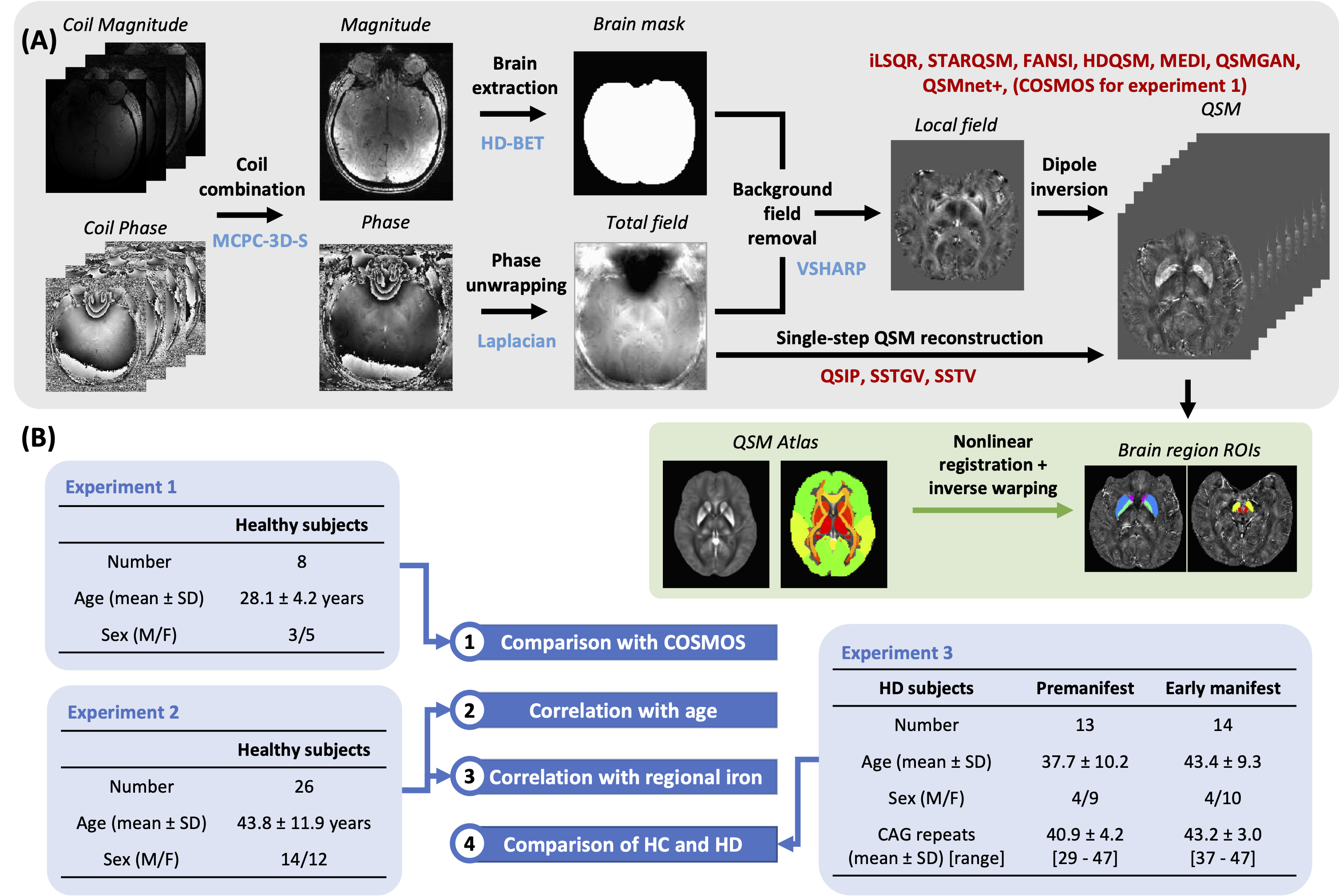
Figure 1. QSM processing pipeline and experiment design. (A) QSM processing pipeline for all subjects. In addition, brain region ROIs were generated for subjects in experiments 2 and 3 by registration of a QSM atlas and predefined whole brain segmentation. The demographics of healthy volunteers and Huntington’s disease subjects who participated in the three experiments were included in (B). SD: standard deviation.
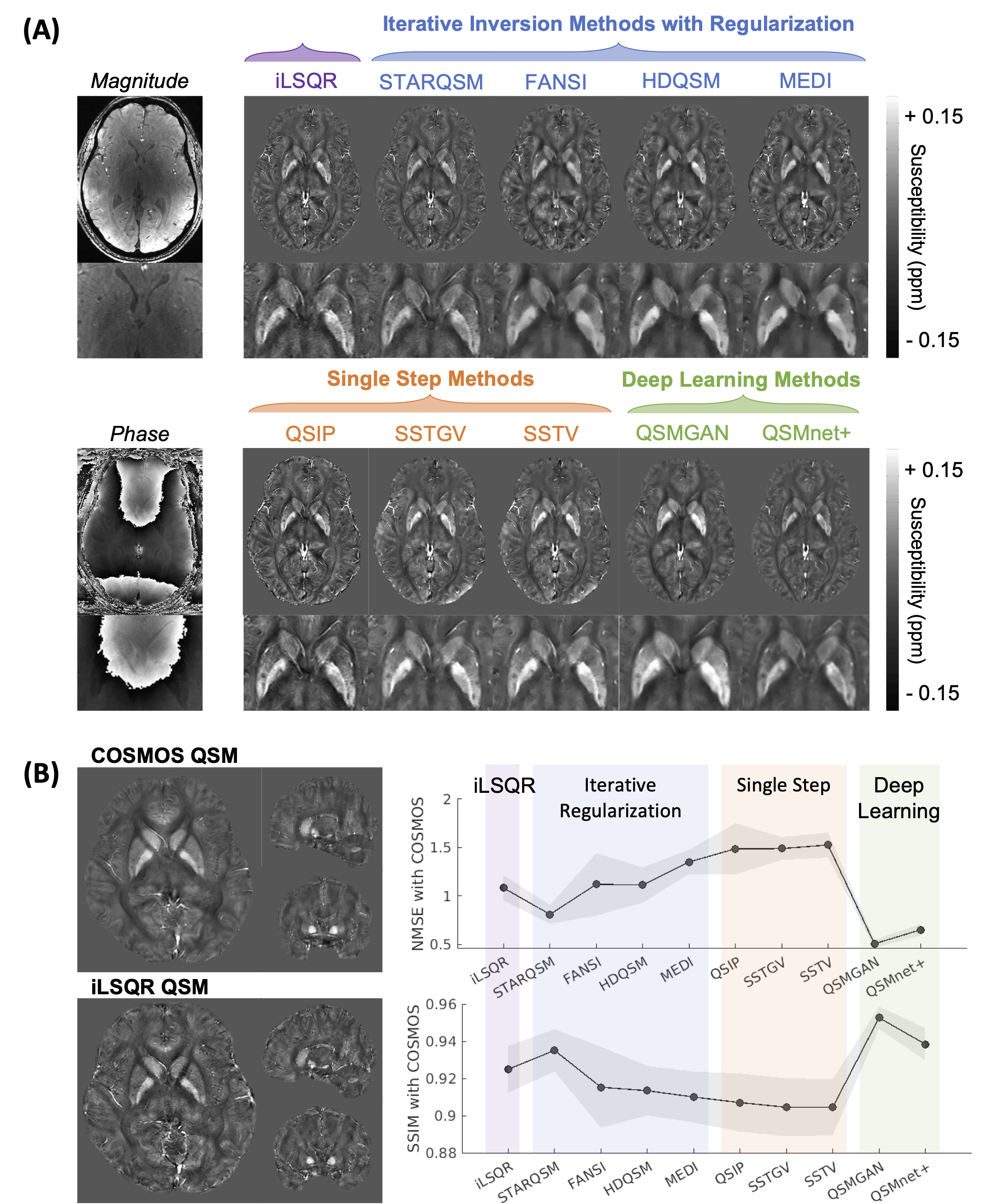
Figure 2. The example QSM images and comparison with COSMOS reference. (A) Example QSM images and the zoom-in depiction on basal ganglia from one healthy volunteer. (B) Example COSMOS and iLSQR QSM images and the NMSE and SSIM plots across all QSM methods. NMSE: normalized mean square error; SSIM: structural similarity index.
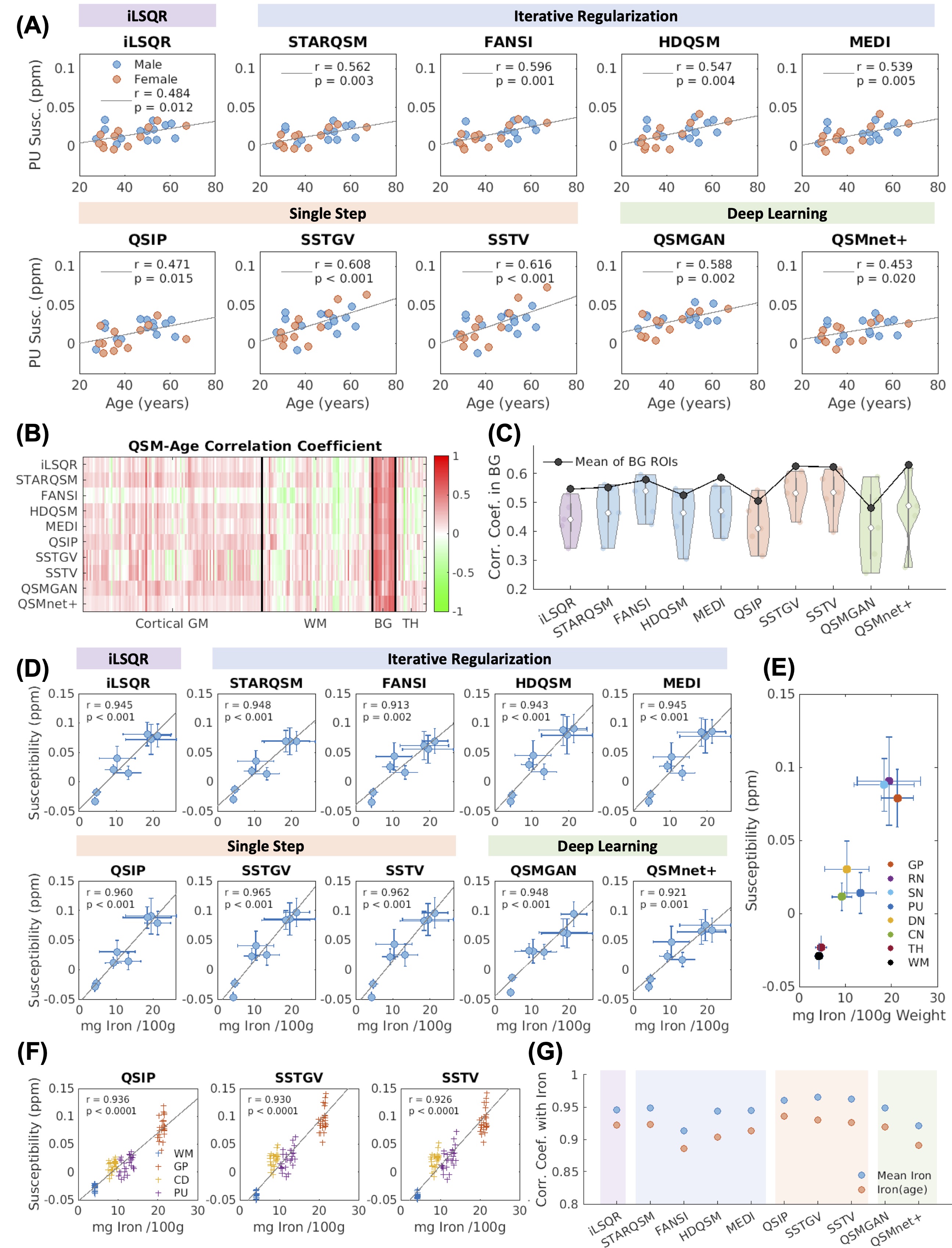
Figure 3. Correlation between QSM values with age and iron. (A) Correlation plots between PU susceptibility and age. (B-C) Correlation coefficients in all brain ROIs and in basal ganglia. (D) Correlations between brain region susceptibility with iron. (E) Brain ROI labels. (F) Correlation between susceptibility with subject-specific iron estimates. (G) Summary of the coefficients in (D) and (F). GM: gray matter; WM: white matter; BG: basal ganglia; TH: thalamus; GP: globus pallidus; RN: red nucleus; SN: substantia nigra; PU: putamen; DN: dentate nucleus; CN: caudate nucleus.
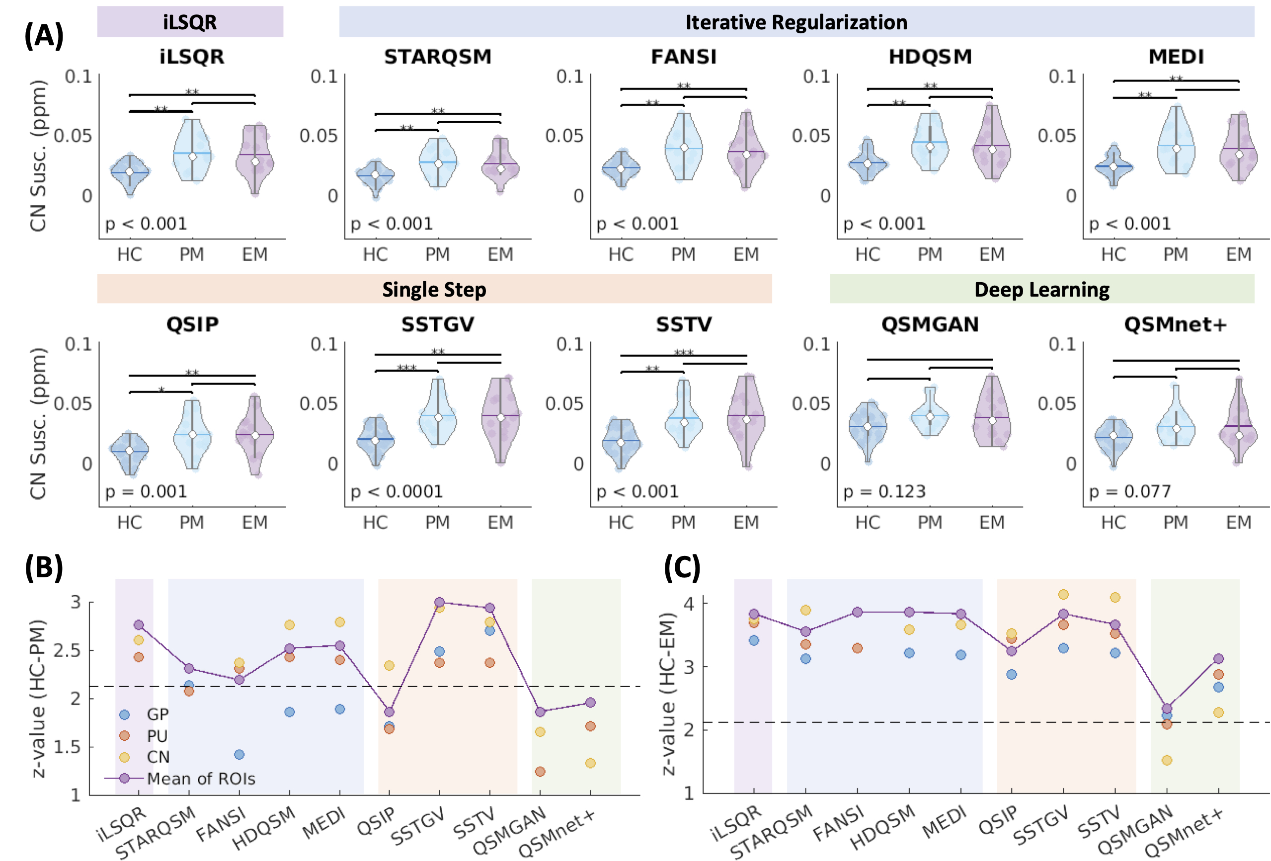
Figure 4. Comparison of QSM values across healthy volunteers, premanifest HD subjects, and early manifest HD patients. (A) The Kruskal-Wallis comparisons of CN susceptibility using different QSM methods across the three groups. (B-C) Test statistics between HC and PM, and between HC and EM. The dotted lines represent the critical value after Dunn’s correction of multiple comparisons. HD: Huntington’s disease; CN: caudate nucleus; HC: healthy control; PM: premanifest HD; EM: early manifest HD; GP: globus pallidus; PU: putamen; *: p < 0.05; **: p < 0.01; ***: p < 0.001.
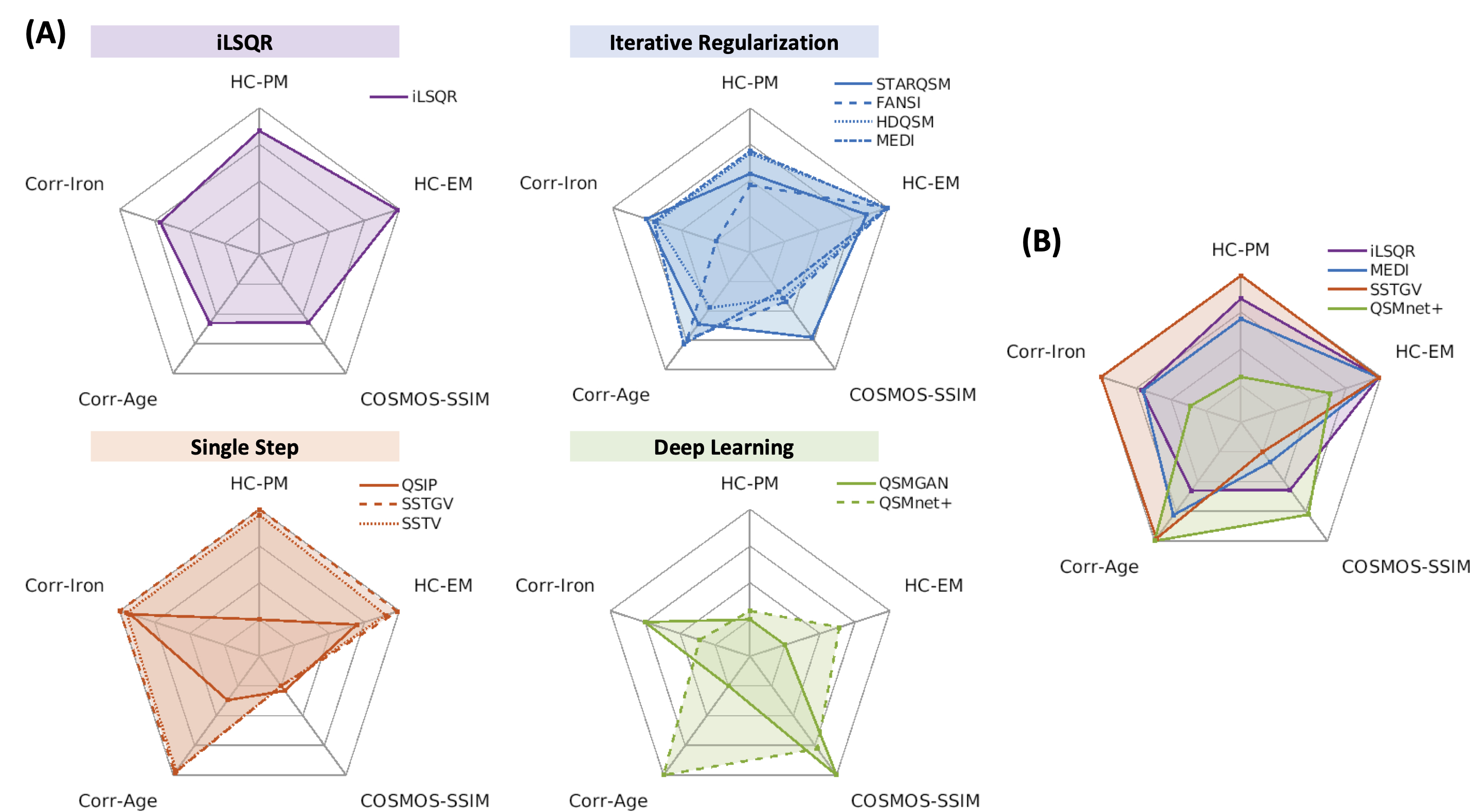
Figure 5. Summary plots of the performance comparison of different QSM methods. Five aspects were included: SSIM compared to COSMOS QSM; correlation coefficient of basal ganglia susceptibility with age; correlation coefficient of mean susceptibility and iron quantification in different brain regions; test statistics of comparison between HC and PM/EM. QSM methods were gathered according to their categories in (A) and one representative method from each group was plotted in (B). HC: healthy control; PM: premanifest HD; EM: early manifest HD; SSIM: structural similarity index.
DOI: https://doi.org/10.58530/2022/2366