Introduction

Susceptibility tensor imaging (STI) is a recent MRI technique that is able to quantify anisotropic magnetic susceptibilities in the human tissues^1–4. STI relies on a least-squares optimization using oversampled data, thus requiring several acquisitions at significantly different orientations to robustly reconstruct each component of a second order tensor. This makes STI particularly difficult in clinical settings. Several methods have been developed to reconstruct the susceptibility tensor with fewer acquisitions, smaller rotation angles, or to improve its robustness against noise (e.g., Mean magnetic susceptibility regularized STI⁵, Diffusion-regularized STI⁶). However, each technique produces significantly different results^5,6. Since there is neither a gold standard for STI reconstructions nor a ground truth, it is difficult to evaluate the accuracy of each technique.
We here describe a realistic in-silico brain phantom for STI, which can be used to evaluate and compare different STI reconstruction methods. We use Diffusion Tensor Imaging (DTI) as prior information to define the STI components, given the similar effects that brain microstructures produce in both STI and DTI ^6,7.

Methods

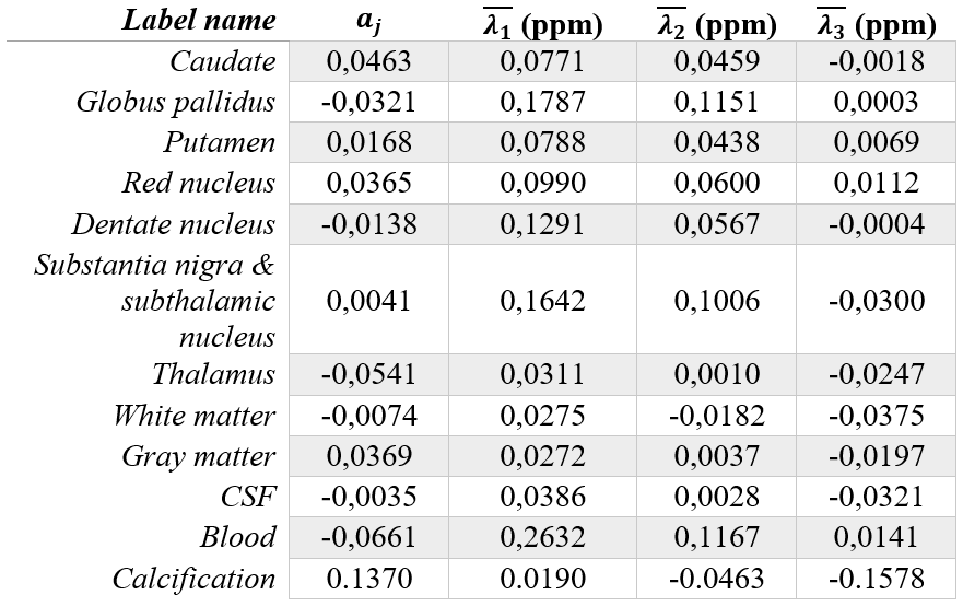
Our STI phantom is inspired in some of the ideas used to create a brain phantom in the context of the QSM Reconstruction Challenge 2.0 (RC2)⁸. We also used data publicly available for that challenge and also from the QSM Reconstruction Challenge 1.0 (RC1)⁹.
We considered a brain composed of 12 structures (Table 1). For each tissue (j), the i-th STI eigenvalue at pixel r $$$(\lambda_{i,j}(r))$$$ was defined as
\begin{equation}
\lambda_{i,j}(r)=\overline{\lambda}_{i,j}(r)+a_j(FA(r)-\overline{FA}_j)\qquad(1)
\end{equation}
where $$$\overline{\lambda}_{i,j}(r)$$$ and $$$\overline{FA}_j$$$ are the mean of the i-th eigenvalue and the mean fractional anisotropy of tissue j, respectively. $$$FA(r)$$$ is the fractional anisotropy at voxel r obtained experimentally from RC2 data. $$$a_j$$$ are weighting factors adjusted empirically. $$$\overline{\lambda}_{i,j}$$$ were set as the mean of the eigenvalues obtained experimentally from RC1 data, considering $$$\lambda_1>\lambda_2>\lambda_3$$$ (Table 1).
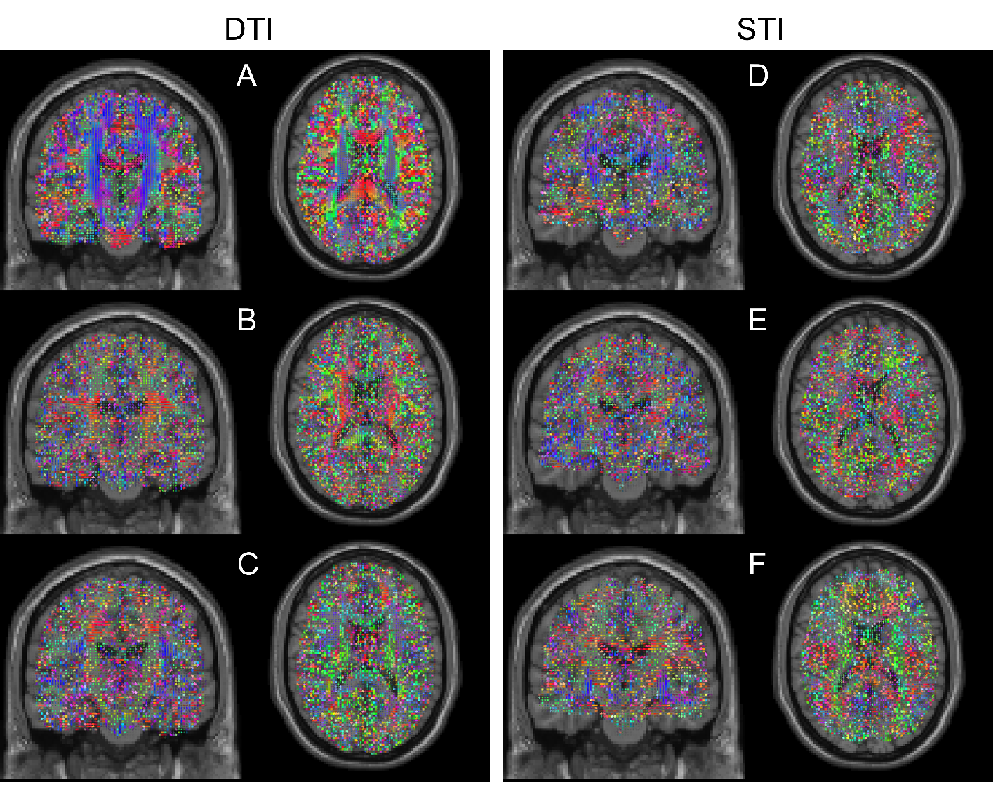
STI and DTI show similar behavior with respect to the fiber bundle direction^6,7 (Figure 1), we derived STI eigenvectors $$$(\nu_1,\nu_2,\nu_3)$$$ from those obtained with DTI data (from RC2). DTI components were filtered using a wavelet denoising algorithm⁸. Subsequently, we performed an eigen decomposition and filtered the resulting eigenvectors using a median filter with a 3×3×3 kernel. Finally, for each voxel r the susceptibility tensor $$$\chi$$$ was computed as in equation 2.
\begin{equation}\chi=\begin{pmatrix}\nu_1 & \nu_2 & \nu_3\end{pmatrix}\begin{pmatrix}\lambda_1&0&0\\ 0&\lambda_2&0\\0&0&\lambda_3\end{pmatrix}\begin{pmatrix}\nu_1^T\\\nu_2^T\\\nu_3^T\end{pmatrix}\qquad(2)\end{equation}

To obtain off-resonant field maps $$$\delta$$$, we estimated the system matrix $$$A$$$ of the tensor^1,2 for five arbitrary rotations and one image without rotation with respect to the main magnetic field (Equation 3 and 4). We set $$$\theta$$$, the angle with respect to the main magnetic field as a random value between 10° and 50°, and $$$\psi$$$, the rotation in the axial plane, as a random value between -50° and 50°.

\begin{equation}\delta=A\hat{\chi}=a_{11}\hat{\chi_{11}}+a_{12}\hat{\chi_{12}}+a_{13}\hat{\chi_{13}} + a_{22}\hat{\chi_{22}}+a_{23}\hat{\chi_{23}}+a_{33}\hat{\chi_{33}}\qquad(3)\end{equation}
$$\begin{matrix}a_{ii}=\frac{1}{3}H_iH_i-\frac{k^T\hat{H}}{k^2}k_iH_i\\a_{ij}=\frac{2}{3}H_iH_j-\frac{k^T\hat{H}}{k^2}(k_i H_j+k_j H_i)\end{matrix}\qquad(4)$$

where $$$\hat{\chi}$$$ is the Fourier Transform of the susceptibility tensor, $$$A$$$ is the matrix projection of the rotation angles inside the scanner, $$$\hat{H}$$$ is the unitary orientation of the main magnetic field. Finally, local phases $$$\phi$$$ were estimated for each simulated orientation by applying the proper phase scale (Equation 5) with $$$\gamma$$$=42.58MHz/T, $$$T_E$$$= 12ms and $$$B_0$$$=7T.
$$
\delta=\frac{\phi}{2\pi{\gamma}T_EB_0}\qquad(5)
$$
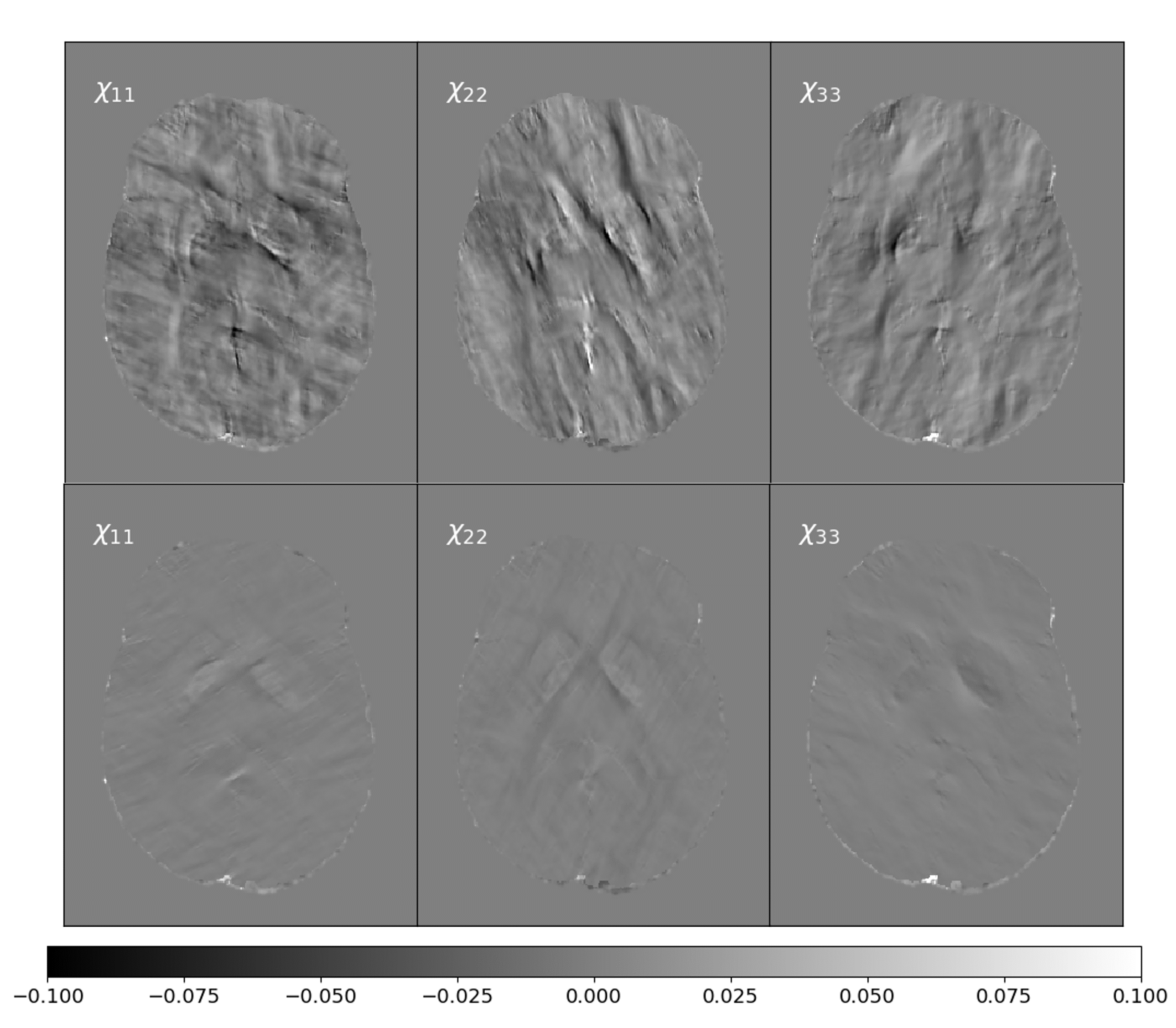
As a proof of concept, we design an experiment to evaluate the effect of noise and number of acquired orientation angles over a least squared STI reconstruction. We built a second phantom considering 12 orientation angles and we compered that STI reconstruction against the one obtained with 6 orientation angles, both phantoms with additive Gaussian noise (with zero mean and standard deviation 1×10^-7) in the local phase.

Results

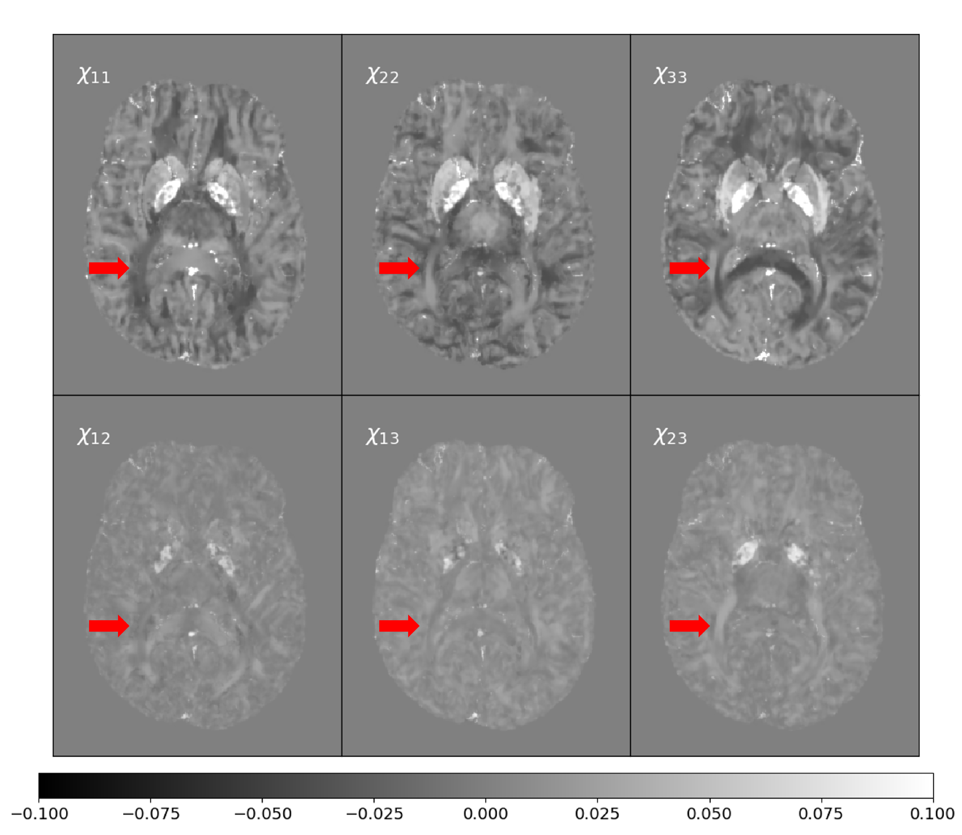
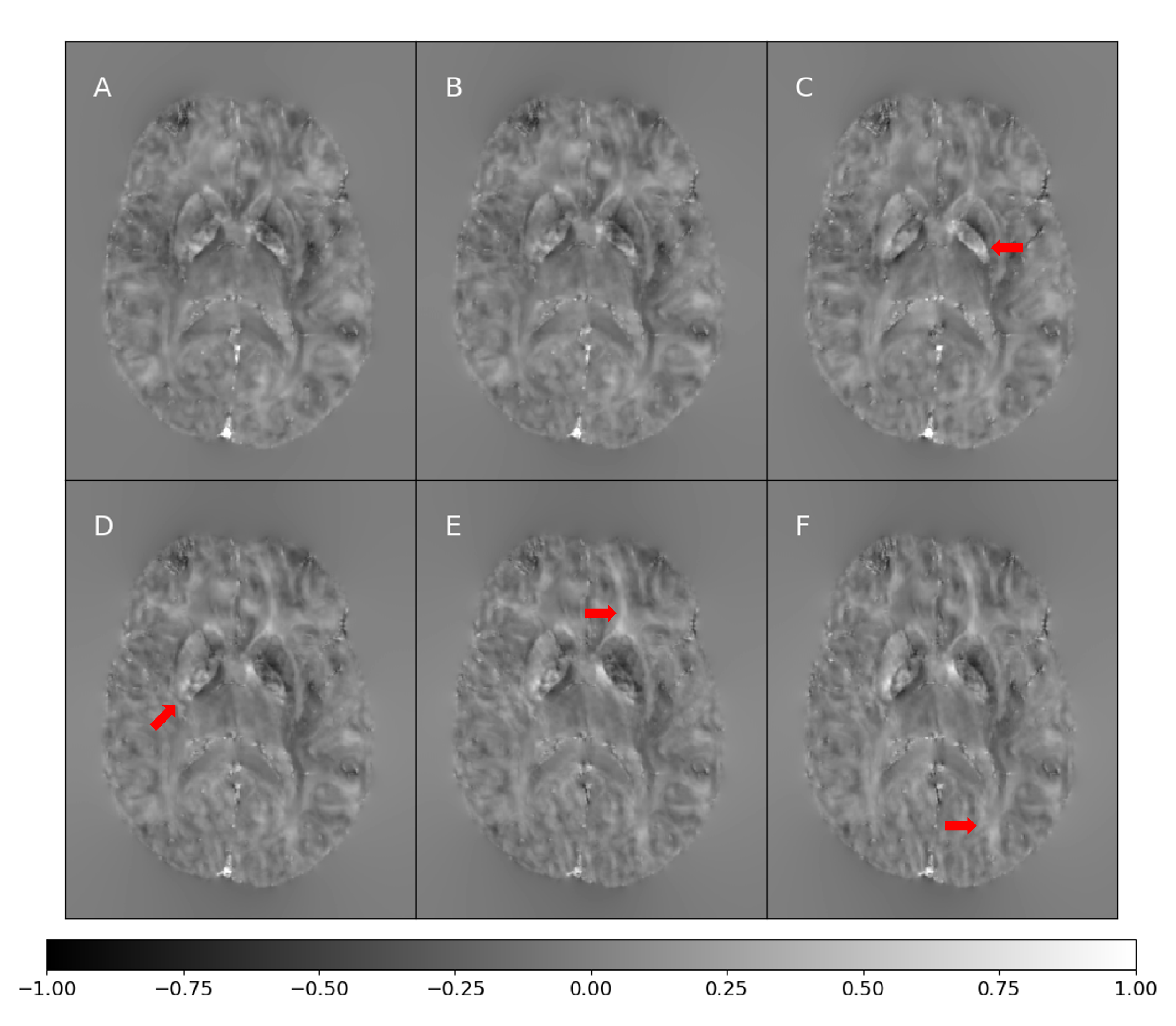
The resulting magnetic susceptibility tensor is shown in Figure 2 with their corresponding local phase images (6 orientation angles) in Figure 3. The phantom successfully shows the anisotropic behavior of susceptibility in white matter areas (red arrows in Figure 2).
Figure 4 shows the difference between the ground truth and the reconstructed STIs for 6 and 12 different orientations angles.

Discussion

Figure 2 show differences in white matter in the reconstructed Tensor. This might be explained by the orientation given by the DTI eigenvectors. Furthermore, isotropic components (Figure 2A- 2C) show more contrast between gray and white matter than anisotropic components, as reported by Liu et al¹⁰ However, anisotropic images appear to be different in images with a high orientation dependency, such as white matter myelin. Such differences in white matter are also present in the local phase (Figure 3).
As expected, the performance of least-square based STI reconstruction methods is affected by noise and the number of acquired orientation angles. Our phantom reproduced a well-known result of such algorithms, namely, reducing the number of acquired orientation angles increases errors in the reconstructed susceptibility tensor values (Figure 4).

Conclusions

We created a realistic phantom for Susceptibility Tensor Imaging (STI). This phantom can be used to evaluate and compare the performance of STI reconstruction methods, and hopefully serve as a tool to design better and more robust STI algorithms.

Acknowledgements

Grant funding Fondecyt 1191710, Anillo PIA ACT192064, Millennium Nucleus for Cardiovascular Magnetic Resonance (NCN17_129). We thank José Marques for sharing imaging data.

References

1. Liu, C. Susceptibility tensor imaging. Magnetic Resonance in Medicine 63, 1471–1477 (2010).

2. Li, W., Liu, C., Duong, T. Q., van Zijl, P. C. M. & Li, X. Susceptibility tensor imaging (STI) of the brain. NMR in biomedicine 30, (2017).

3. Xie, L. et al. Susceptibility tensor imaging of the kidney and its microstructural underpinnings. Magnetic Resonance in Medicine 73, 1270–1281 (2015).

4. Dibb, R., Qi, Y. & Liu, C. Magnetic susceptibility anisotropy of myocardium imaged by cardiovascular magnetic resonance reflects the anisotropy of myocardial filament α-helix polypeptide bonds. Journal of Cardiovascular Magnetic Resonance 17, 60 (2015).

5. Li, X. & van Zijl, P. C. M. Mean magnetic susceptibility regularized susceptibility tensor imaging (MMSR-STI) for estimating orientations of white matter fibers in human brain. Magnetic resonance in medicine 72, 610–619 (2014).

6. Bao, L. et al. Diffusion-regularized susceptibility tensor imaging (DRSTI) of tissue microstructures in the human brain. Medical Image Analysis 67, (2021).

7. Li, W. & Liu, C. Comparison of Magnetic Susceptibility Tensor and Diffusion Tensor of the Brain. J Neurosci Neuroeng 2, 431–440 (2013).

8. Marques, J. P. et al. QSM reconstruction challenge 2.0: A realistic in silico head phantom for MRI data simulation and evaluation of susceptibility mapping procedures. | Berkin Bilgic 3, (2021).

9. Langkammer, C. et al. Quantitative susceptibility mapping: Report from the 2016 reconstruction challenge. Magnetic Resonance in Medicine 79, 1661–1673 (2018).

10. Liu, C., Li, W., Wu, B., Jiang, Y. & Johnson, G. A. 3D fiber tractography with susceptibility tensor imaging. NeuroImage 59, 1290–1298 (2012).