2360
B0 field distortions monitoring and correction for 3D non-Cartesian fMRI acquisitions using a field camera: Application to 3D-SPARKLING at 7T1Université Paris-Saclay, CEA, Neurospin, CNRS, Gif-sur-Yvette, France, 2Université Paris-Saclay, Inria, Parietal, Palaiseau, France, 3Siemens Healthcare SAS, Saint Denis, France, 4Skope Magnetic Resonance Technologies AG, Zurich, Switzerland
Synopsis
The benefit of retrospective correction of static and dynamic $$$B_{0}$$$ field imperfections was studied on non-Cartesian compressed sensing-based acquisition patterns by taking as an example 3D-SPARKLING encoding scheme. Long-TR dynamic acquisitions of T2*-weighted MRI (fMRI-like) volumes were acquired at 7T, retrospectively corrected, and the evaluation of the corrections was based on the image quality and the gain in temporal signal-to-noise ratio (tSNR). We found that correcting for the static and dynamic $$$0^{th}$$$ order contributions is enough to enhance the image quality and tSNR significantly (up to 22% gain in median tSNR).
Introduction
In fMRI, understanding the different sources of confounds and correcting them is an important concern1–3. Magnetic field fluctuations alter the Larmor frequency, hence the nuclear spins phase which encodes the spatial information in MRI. Dynamic field perturbations cause changes in the recorded NMR signal that are unrelated to neuro-vascular coupling and as such can be considered as confounds. Static but spatially varying field distortions are not an issue for the data temporal stability, yet induce signal loss in tissue-air interfaces, especially in non-Cartesian settings and at higher magnetic fields (3T and higher). To address this issue, one can account for static and dynamic $$$B_{0}$$$ perturbations retrospectively in the signal model during image reconstruction4. More specifically, additional measurements can be acquired and used in the extended signal model. The static contribution is usually measured with a $$$B_{0}$$$ map. The dynamic fluctuations can be monitored using navigators but a new method that uses NMR probes5 to monitor the field dynamics concurrently to the imaging process6 was explored in literature for anatomical and functional MRI7–10. Hereafter, we use this NMR probes system, namely the Skope Clip-on Camera, to measure field fluctuations and the actual k-space trajectories to assess the potential benefit of correcting $$$B_{0}$$$ pertubations on 3D-SPARKLING11-13 fMRI-like data at 7T (Fig.1-a).Theory
In a 3D framework, the extended received signal $$$S(t)$$$ model can be written according to the equation below where $$$x(\mathbf{r})$$$ is the density source at the 3D spatial position $$$\mathbf{r}$$$ and $$$\mathbf{k}(t)$$$ is the 3D k-space position at time $$$t$$$. $$$\Delta\text{}B_{0,stat}(\mathbf{r})$$$ reflects the static off-resonance at $$$\mathbf{r}$$$. $$$\Delta\text{}B_{0,dyn}$$$ reflects the global, slowly varying $$$0^{th}$$$ order contribution of the dynamic field fluctuations and is considered constant during a shot. $$$\mathbf{\delta k}(t)$$$ is the dynamic first-order deviation from the nominal position defined by $$$\mathbf{k}(t)$$$. Given measurements of $$$\Delta\text{}B_{0,stat}(\mathbf{r})$$$, $$$\Delta\text{}B_{0,dyn}$$$ and $$$\mathbf{\delta\text{}k}(t)$$$, we can include them in the reconstruction algorithm and have a model that better reflects the actual acquisition process. In a parallel imaging framework, this model is considered for all shots and channels.$$S(t)=\exp{(2\dot{\imath}\pi\Delta\text{}B_{0,dyn}\times\text{}t)}\int_{\mathbf{r}}x(\mathbf{r})\exp{(2\dot{\imath}\pi\Delta\text{}B_{0,stat}(\mathbf{r})\times\text{}t)}\exp{(-2\dot{\imath}\pi(\mathbf{k}(t)+\mathbf{\delta\text{}k}(t))\circ\mathbf{r})}d\mathbf{r}$$
Methods
Acquisition strategy: Functional-like data was collected on a single healthy volunteer at 7T (Siemens Magnetom) using a 1Tx-32Rx Nova head coil with 3D-SPARKLING for the acquisition parameters reported in Fig.1-b. Due to constraints related to the field monitoring system (Skope's Clip-on Camera), the shortest unitary TR we could choose was 150ms. This impacted the volumetric TR. A gradient recalled echo 2D (GRE 2D) sequence with two echoes (Fig.1-b) was used to estimate the $$$B_{0}$$$ map. External sensitivity maps were acquired using a gradient recalled echo (GRE) sequence (Fig.1-b).Common reconstruction strategy: 3D-SPARKLING volumes were reconstructed independently from each other using a nonlinear multi-coil compressed sensing reconstruction that promotes sparsity in the wavelet domain14. The reconstruction was calibrated using the external sensitvity maps. Implementation and details can be found in15-16.
Additional corrections: To correct for the dynamic fluctuations at the $$$0^{th}$$$ order, the raw NMR data needs to be demodulated by $$$-2\dot{\imath}\pi\Delta\text{}B_{0,dyn}\times\text{}t$$$ prior to the reconstruction. The field camera, allows us to measure $$$k_{0}(t)=2\dot{\imath}\pi\Delta\text{}B_{0,dyn}\times\text{}t$$$ at each time point $$$t$$$, thus, we used those measurements for the demodulation. To account for the first-order dynamic field fluctuations, the non-uniform Fourier operator was defined over the measured k-space trajectories (Fig.2). Unlike the Skope system, the scanner applies an Eddy currents compensation phase (ECCPhase) on the recorded signal upon reception. This means that $$$\Delta\text{}B_{0,dyn}$$$ or $$$k_{0}(t)$$$ accounts for Eddy currents-induced fluctuations whereas they are already corrected by the scanner. To be consistent, we retrospectively decompensated the correction applied by the scanner using a simulation of the ECCPhase. Finally, static $$$\Delta\text{}B_{0}$$$ was corrected by including the acquired $$$B_{0}$$$ map in the definition of the extended Fourier operator (see "Theory"), implemeting the method proposed in17. Fig.2 summarizes the data processing pipeline and details the different combinations of corrections that were applied.
Evaluation: The comparisons were based on the impact on image quality (assessed visually) and on the tSNR (an objective and relevant criterion for fMRI).
Results and Discussion
Fig.3-a shows the effect of the different corrections on image quality: The main difference comes from $$$\Delta\text{}B_{0,stat}$$$ correction. Fig.3-b shows that $$$\Delta\text{}B_{0,dyn}$$$ smoothes the mean difference image slightly. Fig.4 and Fig.5-a show, that in terms of tSNR, the highest benefit is achieved when correcting for both dynamic and static contributions (up to 26$$$\%$$$ gain in median tSNR for the best scenario). Additionally, the gain brought by $$$\mathbf{\delta\text{}k}(t)$$$ is modest when compared to $$$\Delta\text{}B_{0,stat}$$$ and $$$\Delta\text{}B_{0,dyn}$$$. However, Fig.5-b shows that an increase in the median tSNR comes with an increase in the standard deviation as well: this needs to be considered carefully. A Mood test between the corrected and uncorrected data proved that the gain in median tSNR is statistically significant.Conclusion
Correcting for $$$\Delta\text{}B_{0,stat}$$$ enhances image quality greatly, pairing it with $$$\Delta\text{}B_{0,dyn}$$$ correction significantly boosts the tSNR. The gain in tSNR when including $$$\mathbf{\delta\text{}k}(t)$$$ in the reconstruction is lesser. We also highlight the limitations :1)The external $$$B_{0}$$$ map constitutes a limitation since patient movement will cause misalignement with the fMRI scans and consequently impact the correction.
2)The current volumetric TR used is too long for a real fMRI application.
This proof of concept will be extended for a better temporal resolution.
Acknowledgements
Leducq Foundation (Large Equipement ERPT program, NEUROVASC7T project) provided financial support for this work. Chaithya G.R. was supported by the CEA NUMERICS program, which has received funding from the European Union’s Horizon 2020 research and innovation program under the Marie Sklodowska-Curie grant agreement No 800945.
References
1 K. Murphy et al. Resting-state fMRI Confounds and Cleanup. Neuroimage, 80:349–59, 2013.
2 M. G. Bright et al. Cleaning Up the fMRI Time Series: Mitigating Noise with Advanced Acquisition and Correction Strategies. Neuroimage, 154:1–3, 2017.
3 C. Caballero-Gaudes et al. Methods for Cleaning the Bold fMRI Signal. Neuroimage, 154:128–149, 2017.
4 Mariya Doneva. Mathematical Models for Magnetic Resonance Imaging Reconstruction. IEEE Signal Processing Magazine, 37(1):24–32, 2020.
5 N. De Zanche et al. NMR Probes for Measuring Magnetic Fields and Field Dynamics in MR Systems. Magnetic Resonance in Medecine, 60(1):176–86, 2008.
6 C. Barmet et al. Spatiotemporal Magnetic Field Monitoring for MR. Magnetic Resonance in Medecine, 60(1):187–197, 2008.
7 L. Kasper et al. Monitoring, Analysis, and Correction of Magnetic Field Fluctuations in Echo Planar Imaging Time Serie. Magnetic Resonance in Medecine, 74(2):396–409, 2015.
8 S.J. Vannesjo et al. Retrospective Correction of Physiological Field Fluctuations in High-field Brain MRI Using Concurrent Field Monitoring. Magnetic Resonance in Medecine, 73(5):1833–1843, 2015.
9 J. M. Schwarz et al. Correction of Physiological Field Fluctuations in High- and Low-resolution 3D-EPI Acquisitions at 7 Tesla. ISMRM, 2019.
10 S. Bollmann et al. Analysis and Correction of Field Fluctuations in fMRI Data Using Field Monitoring. Neuroimage, 154:92–105, 2017.
11 C. Lazarus et al. SPARKLING: Variable-density k-space Filling Curves for Accelerated T2*-weighted MRI. Magnetic Resonance in Medicine, 81(6):3643–3661, 2019.
12 C. Lazarus et al. 3D Variable-density SPARKLING Trajectories for High-resolution T2*-weighted Magnetic Resonance Imaging. NMR in Biomedicine, 33(9), 2020.
13 G.R. Chaithya et al. Optimizing Full 3D SPARKLING Trajectories for High Resolution T2*-weighted Magnetic Resonance Imaging. under review at IEEE Transactions on Medical Imaging, 2021.
14 L. El Gueddari et al. Self-calibrating Nonlinear Reconstruction Algorithms for Variable Density Sampling and Parallel Reception MRI. IEEE 10th Sensor Array and Multichannel Signal Processing Workshop (SAM), 2018.
15 https://github.com/CEA_COSMIC/pysap-mri.
16 S. Farrens et al. Pysap: Python Sparse Data Analysis Package for Multidisciplinary Image Processing. Astronomy and Computing, 32, 2020.
17 J. A. Fessler et al. Toeplitz-based Iterative Image Reconstruction for MRI with Correction for Magnetic Field Inhomogeneity. IEEE Transactions On Signal Processing, 53(9):3393–3402, 2005.
18 L. El Gueddari et al. Calibrationless Oscar-based Image Reconstruction in Compressed Sensing Parallel MRI. IEEE 16th International Symposium on Biomedical Imaging, 2019.
Figures
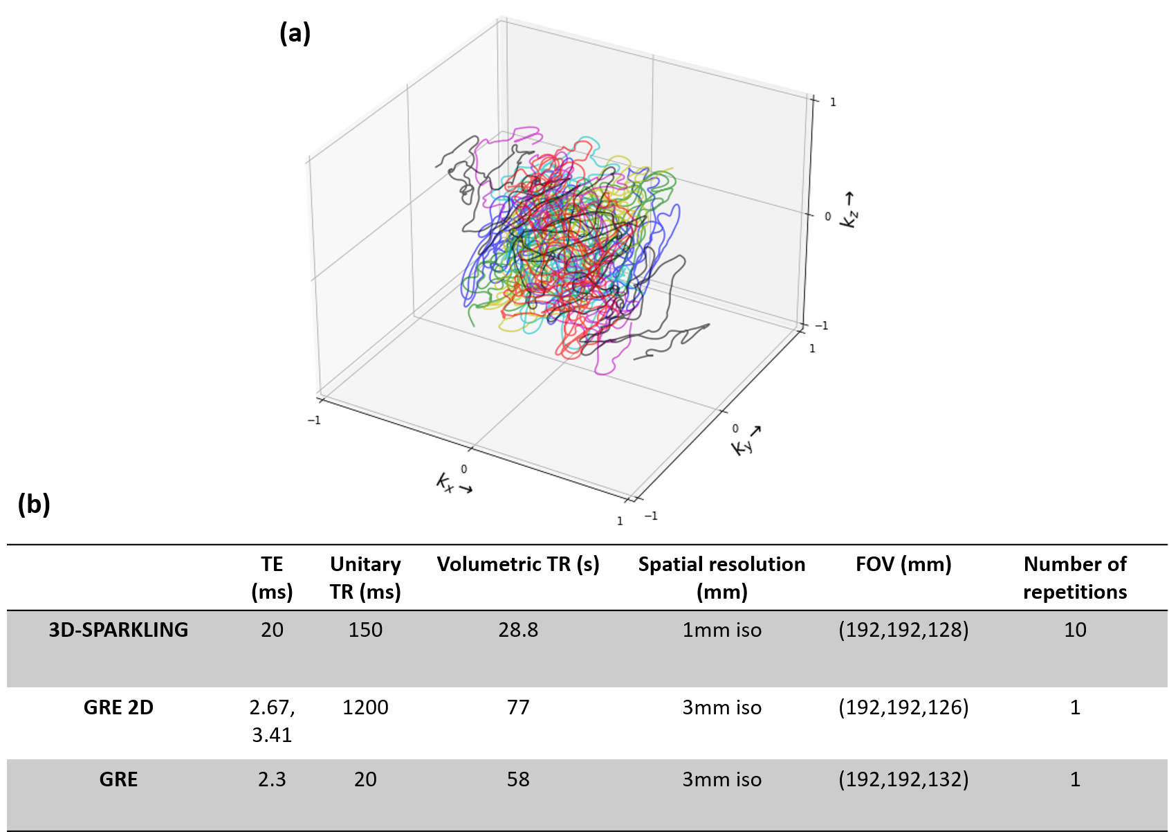

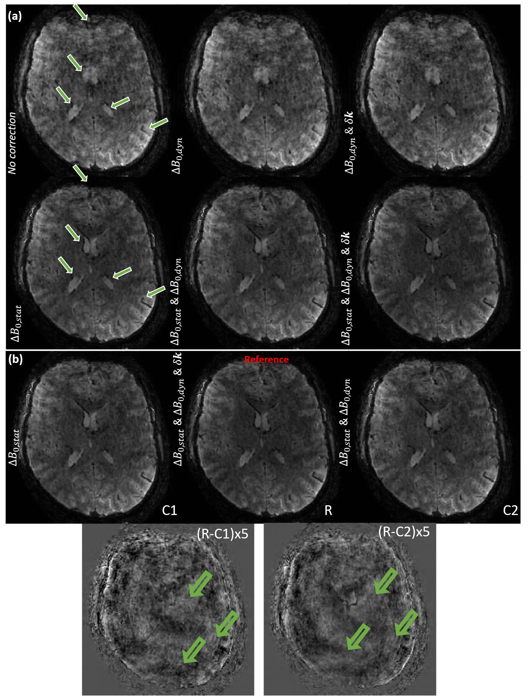


Fig.5: (a) A table summarizing the gain in median tSNR (in $$$\%$$$) for the different correction setups. (b) Boxplot of the relative change in tSNR in $$$\%$$$ compared to the native (no correction) tSNR computed over the 3D masked brain. A Mood test proved that the native (no correction) median tSNR is significantly improved (at a statistical level of significance of $$$10^{-3}$$$) with the five different corrections implemented.