Introduction

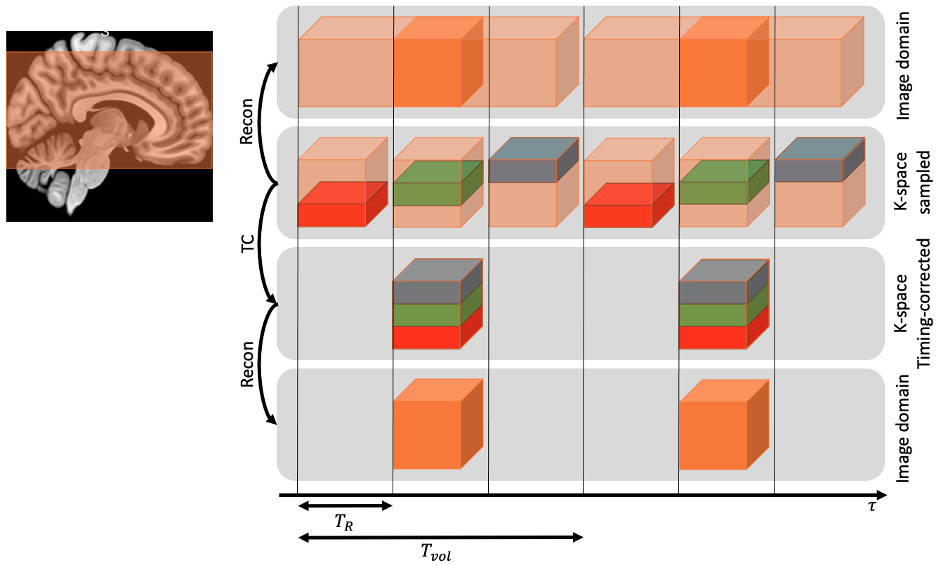
Timing correction (TC) for 2D imaging has been addressed¹ by assuming that the timeseries of a voxel in image space is sufficiently bandlimited such that fulfils the Nyquist criterion. Slices which were acquired at different points in time are temporally shifted such that each volume becomes consistent w.r.t time, commonly known as “slice timing correction²”. For 3D sequences, it is not immediately clear how to achieve TC in image domain. Through the reconstruction, signal timing is “smeared” over the whole volume repetition time. This is exemplary shown in the upper part of Figure 1 for a 3D EPI³. However, if it can be assumed that timeseries of voxels are bandlimited in image domain, the same property holds in k-space. Hence, TC can be achieved in k-space by sinc interpolation. We investigate the veracity of this idea. Additionally, we describe how TC in k-space affects the reconstructed images and quantify the effects of TC on image timeseries.

Methods

The magnetization dynamic at location $$$r$$$ during the readout may be modeled as $$\rho(r)e^{-t/T_2^*(r,\tau)}$$
$$$\rho(r)$$$is the initial magnetization and $$$T_2^*$$$ the effective transverse magnetization decay. $$$t\in[0,T_R]$$$ is the intra-shot time, and $$$\tau$$$ the inter-shot time. We assume that the expression above is bandlimited w.r.t $$$\tau$$$ such that T_vol (see Figure 1) fulfils the Nyquist criterion. This property is not altered by spatial encoding, enabling sinc interpolation k-space. All data were acquired by running a 3D EPI sequence at 3T (FOV: 198x198x125mm ang. 20° backwards, Res.: 2.5mm iso., R:2x2, T_vol=2s, T_E=30ms, T_R=67ms, Flip-angle:19.24°, 600 dynamics). The subject performed an event-related task with stimulation in the upper and lower visual field (UVF and LVF). In total, 400 stimuli were presented with randomly jittered onsets.
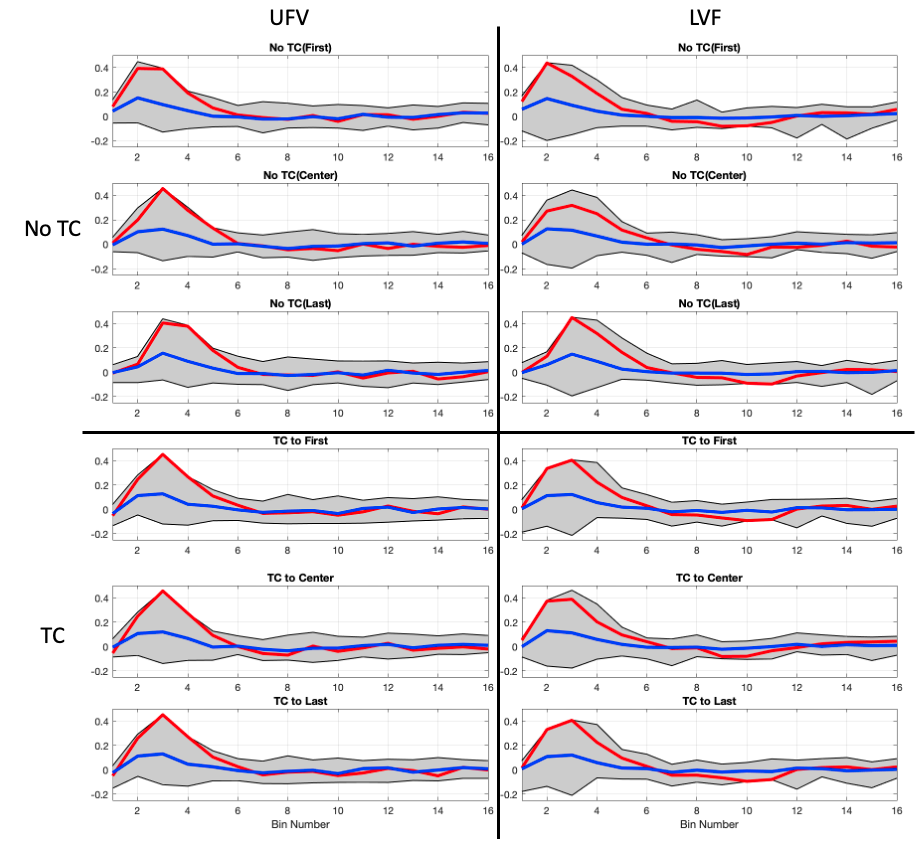
We applied TC three times, shifting all parts of k-space to coincide temporally with the first, central, and last shot. Subsequently, a GLM analysis (SPM12) was run using a FIR basis set3 (16bins, 32s duration). We sampled the regressors in accordance with the TC and compare the computed β-estimates to those obtained without TC. Timing inconsistencies between regressors and data should be captured by this measure.
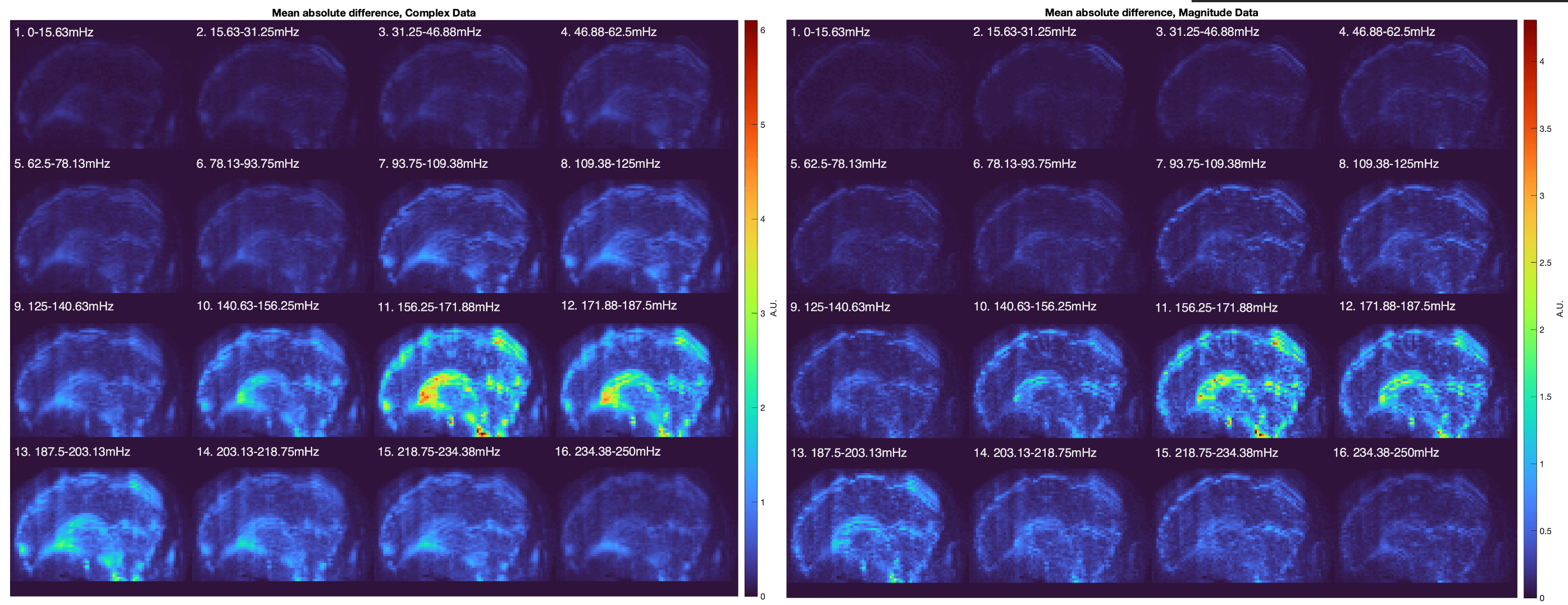
High-frequency components of k-space timeseries should experience a stronger intra-volume change by sinc interpolation than low-frequency components. Therefore, inconsistent timing of high-frequency components of k-space timeseries should result in stronger artifacts in image domain. To investigate this effect, we applied 16 bandpass filters before TC. The filters split the resolvable spectrum (±0.25Hz) into bands of equal width (15.63mHz). The mean absolute difference over time was computed between images with and without TC and for each frequency band. This analysis was restricted to 256 dynamics to reduce the computational burden.
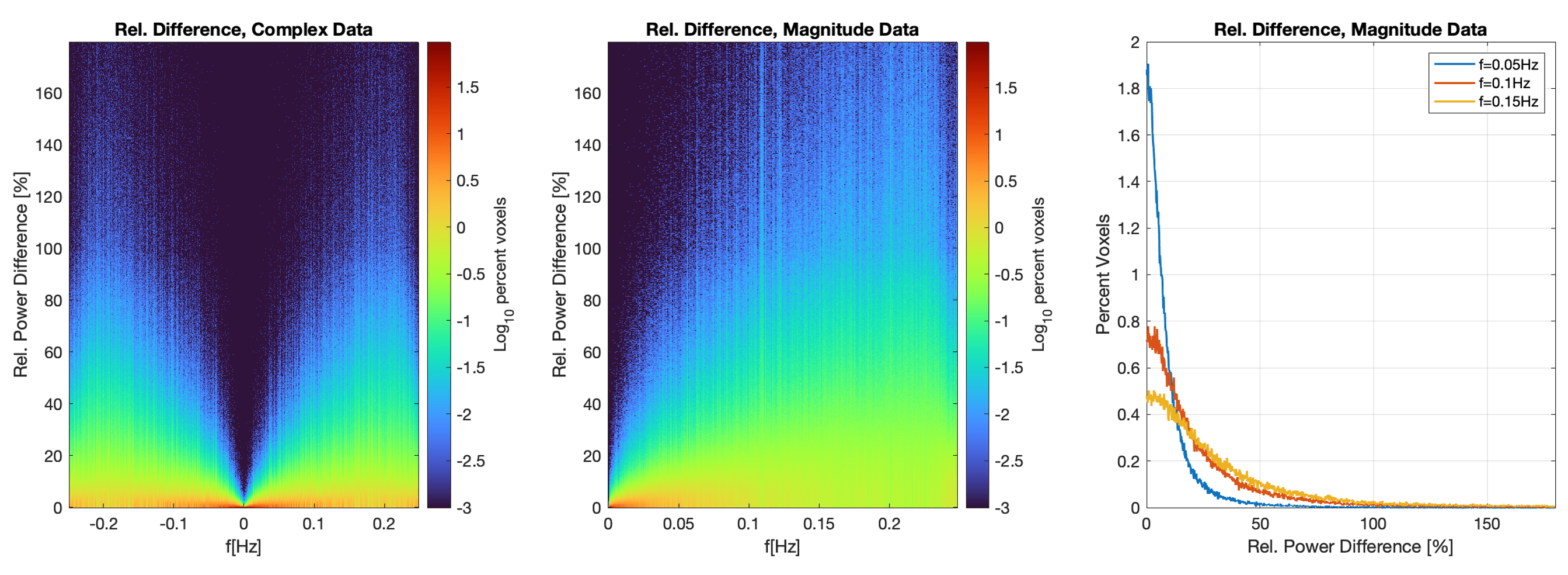
Effects on image domain timeseries were assessed by comparing power spectra of voxel timeseries. For comparability, we normalized them to unit signal energy and computed for each frequency a histogram of absolute percent change in power due to TC.

Results

Figure 2 shows the fitted β-estimates. In the top three rows, TC was not applied but the sampling of the regressors was varied. The complementary estimates with TC are shown in the bottom three rows. TC yields much more consistent results. In both cases, UVF and LVF, temporal shifts in the estimates are reduced due to TC.
The mean absolute difference over time is depicted for all frequency bands in Figure 3. The comparison is made for complex and magnitude images. The spatial artefact caused by the timing problem becomes well visible with increasing frequency and is also preserved after applying the magnitude operator.
Histograms of relative differences in the power spectrums are shown in Figure 4. It is more likely that signal power at high frequency experiences a strong relative change. For instance, at 0.05Hz most voxels experience a change of less than 20% in power, at 0.15Hz many voxels experience a much stronger change.

Discussion

The FIR estimates in Figure 2 show that TC in k-space actually works as intended. It is clear that TC has the intended effect on the timing of the data.
The strength of the spatial artefact increases with frequency of k-space timeseries, peaking in the 11^th band (see Figure 3). Streaking patterns in z-direction of the FOV are visible. Since for a 3D EPI the through-slab direction solely depends on $$$\tau$$$ these artefacts appear in z-direction. The peak in the 11^th band can be explained by lots of signal power in this band (possibly related to respiration) and the finite length of the used interpolation kernel which shifts its cutoff slightly away from 0.25Hz, reducing the effect in the subsequent bands.
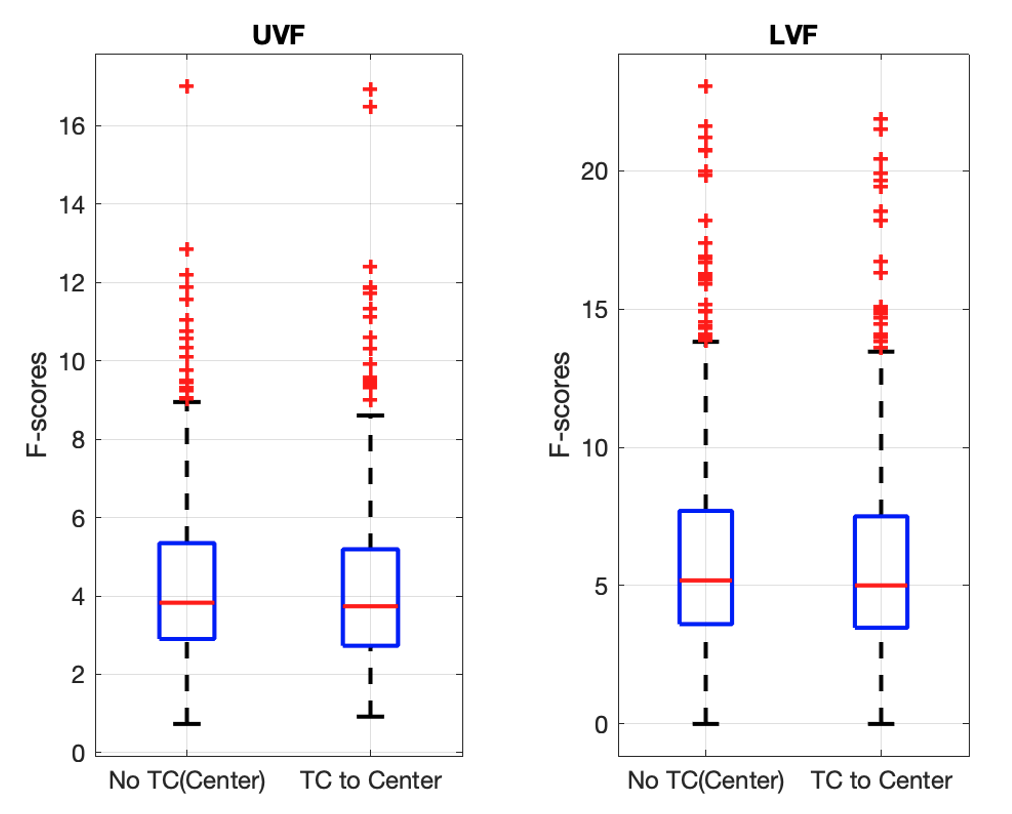
Power at high frequencies of image timeseries is likely to experience a stronger relative change due to TC. The closer spectral components of timeseries lie to the border of the resolvable spectrum the stronger the effect of TC. Figure 5 shows that the statistics of our GLM analysis have barely been altered. One possible explanation could be that low-frequency components as modeled by the HRF are not strongly altered.

Conclusion

We have demonstrated TC for 3D EPI sequences. Artefact strength in space increases with temporal frequency of k-space timeseries. High-frequency components of timeseries in image domain are altered strongly by TC.

Acknowledgements

No acknowledgement found.