2237

Numerical simulation of wave propagation through interfaces using the eXtended FEM for MR elastography

Quanshangze DU¹, Simon Auguste LAMBERT², Nahiène HAMILA³, and Aline BEL-BRUNON¹
¹Univ Lyon, INSA Lyon, CNRS, LaMCoS, UMR5259, 69621 Villeurbanne, France, ²Université de Lyon, INSA Lyon, Université Claude Bernard Lyon 1, Ecole Centrale de Lyon, CNRS, Ampère UMR5005, Villeurbanne, France, ³ENI Brest, UMR CNRS 6027, IRDL, F-29200 Brest, France

Synopsis

The finite element method (FEM) is widely used for modeling wave propagation and stiffness reconstruction in magnetic resonance elastography (MRE). However, it is not that efficient for modeling inclusions with complex interfaces. Here, we propose a formulation of FEM known as the eXtended FEM (XFEM), and investigate this method in two studies: wave propagation across an oblique linear interface and stiffness reconstruction of a random-shape inclusion. XFEM results present good agreement with the theoretical predictions and FEM simulation results. XFEM can be regarded as an ideal alternative to FEM for inclusion modeling in MRE.

Introduction

Magnetic resonance elastography (MRE) is an elasticity imaging technique to quantitatively assess the stiffness of human tissues.¹ Stiffer zones could represent lesions such as tumors and fibroses.² To reconstruct the stiffness distribution based on the wave measurement, the finite element method (FEM) is widely used to model the wave propagation within tissues.³ However, for modeling complex inclusion in FEM, the mesh has to conform with the interface, which often requires a finer mesh leading to increasing computation time. Furthermore, the wave mode conversion is usually neglected and under study in the literature.^4,5 The purpose of this work is to present a formulation of FEM, i.e. the eXtended FEM (XFEM), in MRE simulations. Using XFEM, the wave conversion across a linear interface between two viscoelastic materials is first studied, and a random-shape inclusion is then modeled and reconstructed. Comparisons with theoretical and FEM results are performed and demonstrate the advantages of XFEM.

Methods

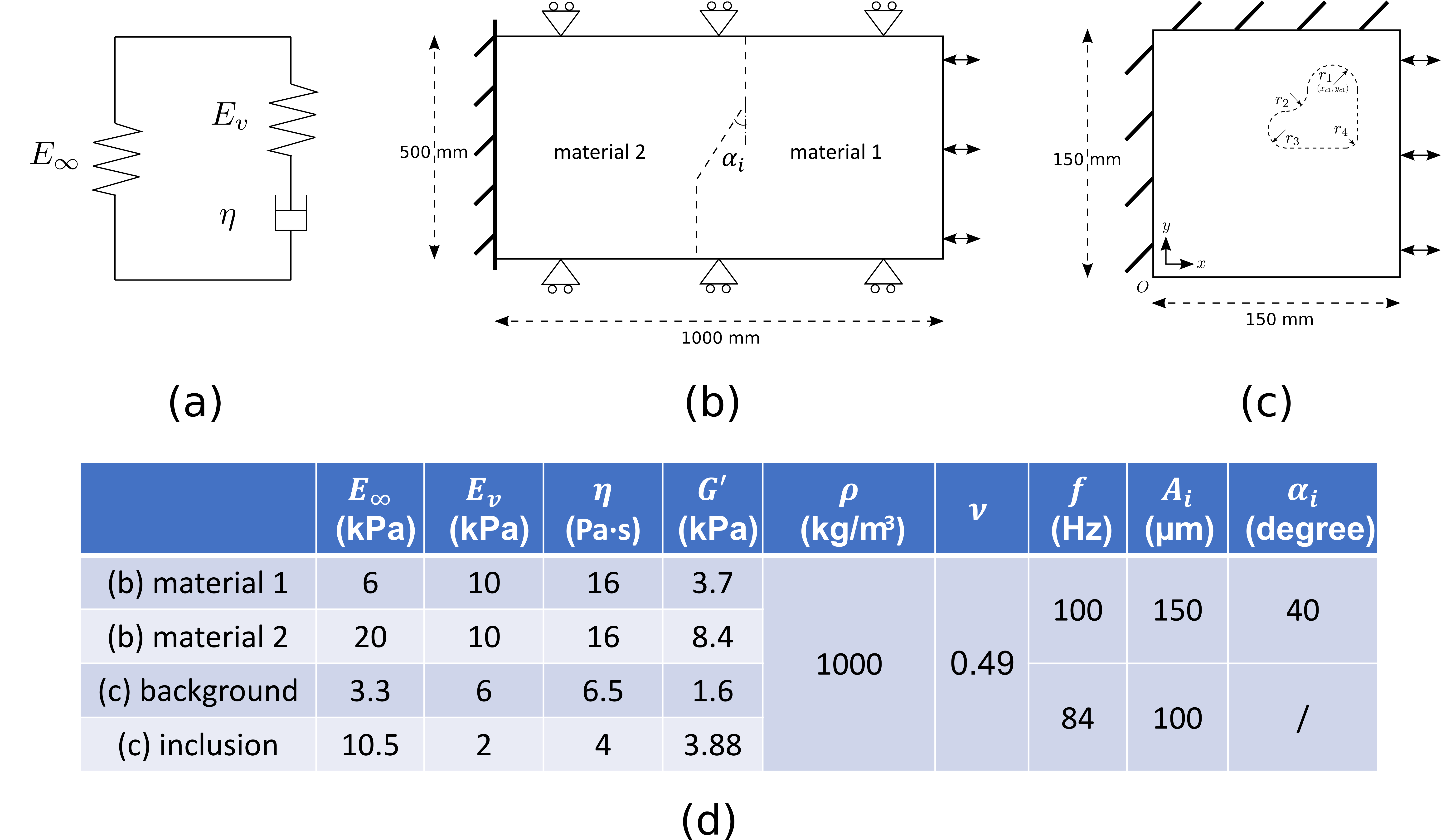
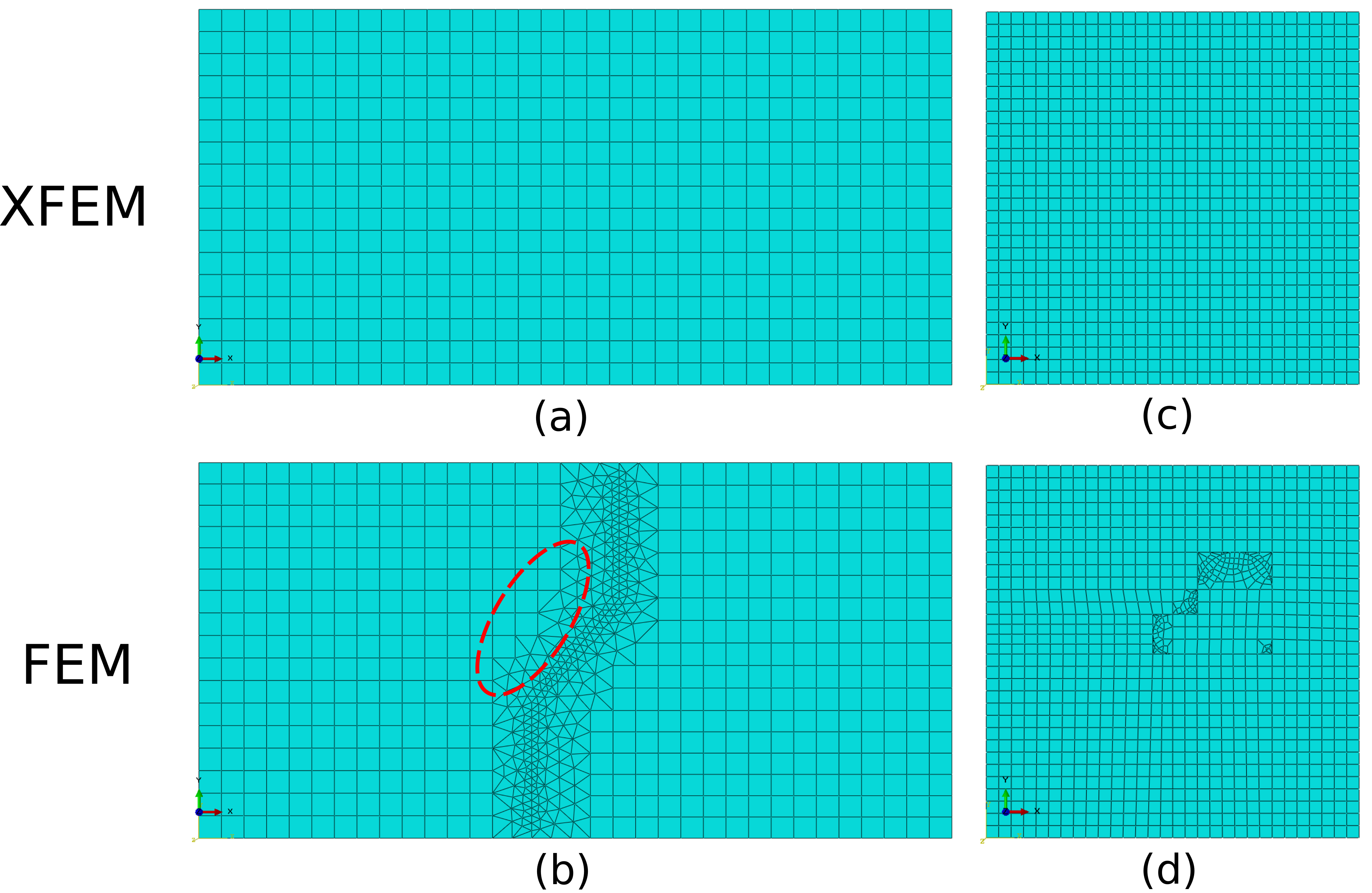
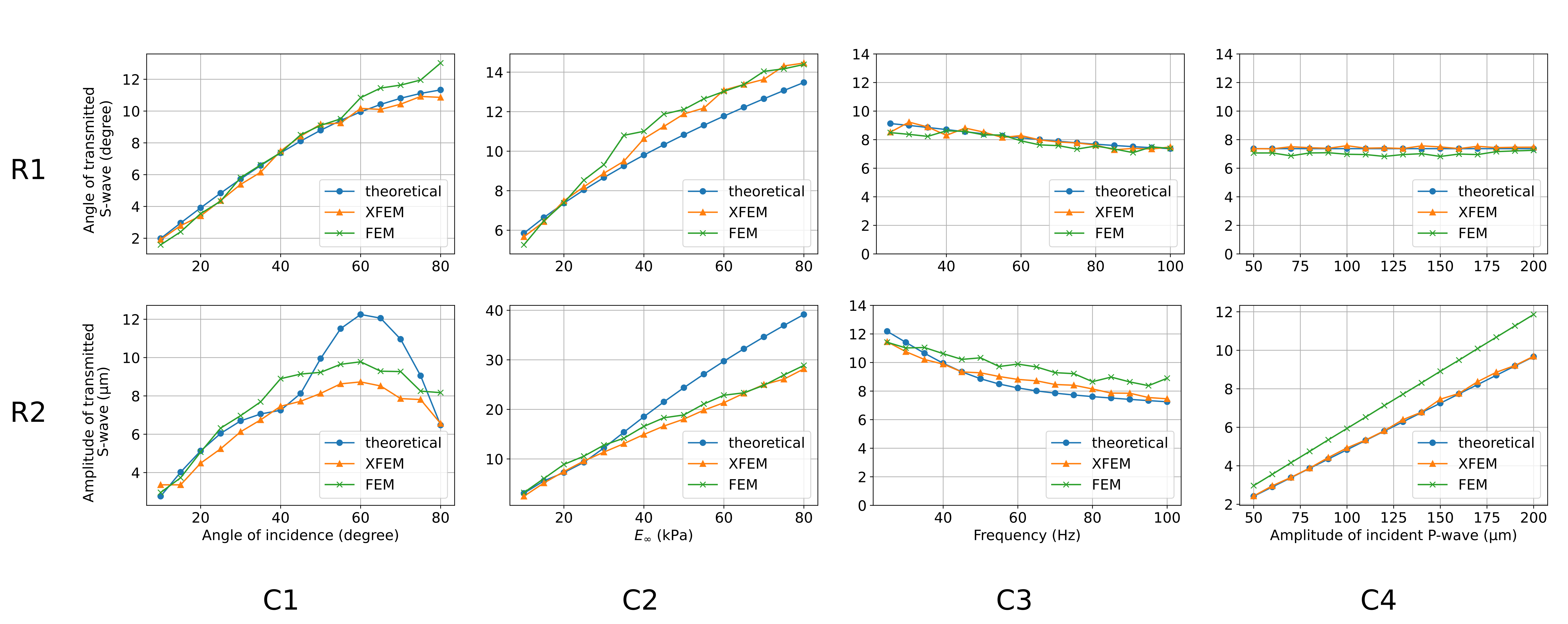
XFEM was initially proposed for crack evolution modeling in fracture mechanics.⁶ It can be also applied for inclusions and voids.⁷ The key idea is to enrich the elements in the vicinity of interface by adding degrees of freedom; the interface becomes independent of the mesh and does not require mesh refinement. We have implemented XFEM/FEM in a homemade explicit solver in Fortran for modeling mechanical wave propagation in a linear, viscoelastic, isotropic and locally homogeneous medium. The standard linear solid model (Fig 1a) was used for describing viscoelasticity.

A case of plane compressional waves (P-waves) crossing an oblique linear interface was first studied in 2D under plane strain hypothesis, as depicted in Fig 1b, by XFEM (Fig 2a) and FEM (Fig 2b). The transmitted shear waves (S-waves) were measured in terms of angle of refraction $$$\alpha_t$$$ and amplitude $$$A_t$$$. The influence of angle of incidence $$$\alpha_i$$$ (10 to 80 degrees), Young's modulus $$$E_{\infty}$$$ (10 to 80 kPa), excitation frequency $$$f$$$ (25 to 100 Hz) and excitation amplitude $$$A_i$$$ (50 to 200 µm) on $$$\alpha_t$$$ and $$$A_t$$$ was evaluated. A related theoretical work⁸ was used for validating the numerical results.

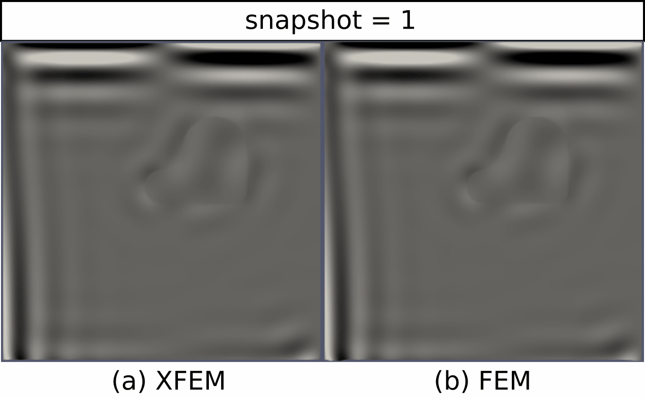
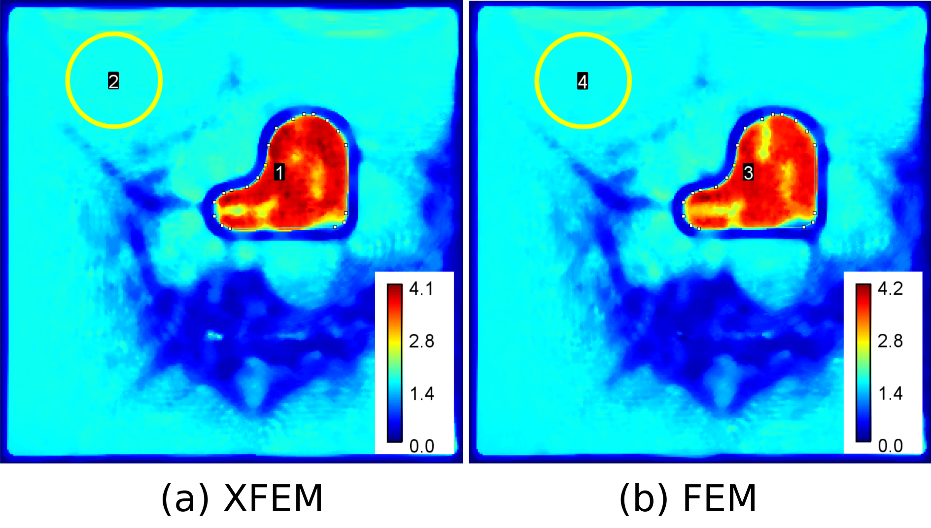
In addition, a square model with a random-shape inclusion, as shown in Fig 1c, was developed in a pseudo-practical application. It was modeled by XFEM (Fig 2c) and compared to standard FEM (Fig 2d). A regular mesh with 300x300 quadrilateral elements was used for the XFEM simulation, while the FEM model was partitioned for a mixed mesh with 90582 quadrilateral and 92 triangle elements. The simulations were executed for 100 harmonic periods with a time-step of 7.44 microseconds on a Linux cluster (running CentOS Linux 7.9.2009) with three CPUs Intel(R) Xeon(R) CPU Gold 5118 @ 2.30 GHz and 5GB RAM. The shear components of converted displacement $$$u_T$$$ were extracted using the curl-operator⁹ and processed with the AIDE algorithm¹⁰ implemented in the MREJ tool¹¹ for reconstructing shear modulus $$$G'$$$.

The related parameters are listed in Fig 1d.

Results and discussion

For the first model, the results of $$$\alpha_t$$$ and $$$A_t$$$ of transmitted S-waves from XFEM/FEM simulation and theoretical prediction are presented in Fig 3. As can be seen, there are differences in some cases between numerical and theoretical results, especially for large angles of incidence $$$\alpha_i$$$ (Fig 3: R2-C1) and great values of $$$E_{\infty}$$$ (Fig 3: R2-C2). Indeed, these offsets are due to the effects of corner which is between oblique and vertical segment of interface. However globally, the XFEM simulations match well with the FEM results, and even perform better when compared to the theoretical predictions. For example, in Fig 3: R2-C4, XFEM agrees with the theory much better than FEM.

For the second model, the results of $$$u_T$$$ and $$$G’$$$ are illustrated in Fig 4 and 5, respectively, both with the methods of XFEM and FEM. It takes around 7 hours for both simulations. Indeed, using XFEM could be time-saving for complex interface requiring more delicate mesh for FEM model. In terms of $$$u_T$$$ fields, the 8 snapshots were taken from a period in steady state (100th period). Qualitatively from the animation, XFEM presents a fairly good agreement with FEM. In terms of $$$G’$$$ fields, the modulus of inclusion is estimated at 3.433±0.500 kPa from XFEM results and 3.325±0.539 kPa from FEM results, with the ground-truth value being 3.88 kPa. The modulus of background, evaluated within a circular region, is estimated at 1.596±0.021 kPa from XFEM results and 1.597±0.015 kPa from FEM results, with the ground-truth value being 1.6 kPa. Quantitatively, compared to the FEM model, the XFEM model gives rise to similar, even better reconstruction results.

Through these two studies, XFEM presents its potential and is expected to be employed in more applications such as the stiffness reconstruction by artificial neural networks^4,12 for readily generating various and reliable simulated data.

Conclusion

XFEM was proposed in this work for modeling heterogeneity in MRE studies. The wave conversion across an oblique linear interface was investigated numerically and theoretically. A square model containing a random-shape inclusion was developed to compare XFEM with FEM. The results show that XFEM performs as well as FEM and could be a better choice and a promising tool for inclusion modeling in MRE, due to its convenience, speed and accuracy.

Acknowledgements

No acknowledgement found.

References

1. Muthupillai, R. et al. Magnetic resonance elastography by direct visualization of propagating acoustic strain waves. Science 269, 1854-1857 (1995).

2. Glaser, K. J. et al. Review of MR elastography applications and recent developments. Journal of Magnetic Resonance Imaging 36, 757-774 (2012).

3. Honarvar, M. et al. A comparison of direct and iterative finite element inversion techniques in dynamic elastography. Physics in Medicine & Biology 61, 3026 (2016).

4. Scott, J. M. et al. Artificial neural networks for magnetic resonance elastography stiffness estimation in inhomogeneous materials. Medical Image Analysis 63, 101710 (2020).

5. Lilaj, L. et al. Inversion-recovery MR elastography of the human brain for improved stiffness quantification near fluid–solid boundaries. Magnetic Resonance in Medicine 86, 2552-2561 (2021).

6. Moës, N. et al. A finite element method for crack growth without remeshing. International Journal for Numerical Methods in Engineering 46, 131-150 (1999).

7. Sukumar, N. et al. Modeling holes and inclusions by level sets in the extended finite-element method. Computer Methods in Applied Mechanics and Engineering 190, 6183-6200 (2001).

8. Henry, F. & Cooper, Jr. Reflection and transmission of oblique plane waves at a plane interface between viscoelastic media. The Journal of the Acoustical Society of America 42, 1064-1069 (1967).

9. Sinkus, R. et al. Viscoelastic shear properties of in vivo breast lesions measured by MR elastography. Magnetic Resonance Imaging 23, 159-165 (2005).

10. Oliphant, T. E. et al. Complex-valued stiffness reconstruction for magnetic resonance elastography by algebraic inversion of the differential equation. Magnetic Resonance in Medicine 45, 299-310 (2001).

11. Xiang, K. et al. MREJ: MRE elasticity reconstruction on ImageJ. Computers in Biology and Medicine 43, 847-852 (2013).

12. Murphy, M. C. et al. Artificial neural networks for stiffness estimation in magnetic resonance elastography. Magnetic Resonance in Medicine 80, 351-360 (2018).

Figures

Figure 1. Illustration of the standard linear solid (SLS) model (a), the model containing an oblique linear interface (b) and the model with a random-shape inclusion (c). The table (d) presents the default parameters of parametric studies using model (b) and the parameters of model (c). For model (c), the inclusion is characterized by ($$$x_{c1}$$$, $$$y_{c1}$$$) = (110, 110) mm, ($$$r_1$$$, $$$r_2$$$, $$$r_3$$$, $$$r_4$$$) = (15, 10, 8, 6) mm.

Figure 2. Illustration of difference between XFEM and FEM in terms of mesh. (a) and (b) presents the XFEM and FEM mesh, respectively, for the model containing an oblique linear interface. (c) and (d) illustrates the XFEM and FEM mesh, respectively, for the model containing a random-shape inclusion. For illustration purpose, meshes are here much coarser than those used in numerical simulations. The red dashed ellipse in (b) roughly refers to the zone where the measurements of angle $$$\alpha_t$$$ and amplitude $$$A_t$$$ in parametric studies are performed.

Figure 3. Results of parametric studies presenting the variation of angle of refraction $$$\alpha_t$$$ (row R1) and amplitude $$$A_t$$$ (row R2) of transmitted S-waves across an oblique linear interface, in terms of the parameters including angle of incidence $$$\alpha_i$$$ of incident P-waves (column C1), modulus $$$E_{\infty}$$$ of material 2 (column C2), excitation frequency $$$f$$$ (column C3) and amplitude $$$A_i$$$ of incident P-waves (column C4).

Figure 4. Animation of 8 snapshots during a period in steady state (100th period) of curl-applied displacement fields $$$u_T$$$ from the model containing a random-shape inclusion. (a) corresponds to the results of XFEM simulation, while (b) is obtained using the classical FEM.

Figure 5. Results of shear modulus $$$G'$$$ reconstruction from the curl-applied displacement fields of the model containing a random-shape inclusion using the method of XFEM (a) and FEM (b). By XFEM, $$$G'$$$ is estimated at 3.433±0.500 kPa for inclusion (zone 1) and 1.596±0.021 kPa for background (zone 2). By FEM, $$$G'$$$ is estimated at 3.325±0.539 kPa for inclusion (zone 3) and 1.597±0.015 kPa for background (zone 4). The ground-truth value of $$$G'$$$ is 3.88 kPa for inclusion and 1.6 kPa for background.

Proc. Intl. Soc. Mag. Reson. Med. 30 (2022)

2237

DOI: https://doi.org/10.58530/2022/2237