Introduction

Gradient-echo line-scanning (GELINE) fMRI is a recent technique^1,2 able to achieve extremely high spatio-temporal resolution in one direction (250 μm and 105 ms, in humans), at the cost of volume coverage. Subject movement leads to image artifacts but this is even more problematic at high resolution MRI, where smaller movements also have an impact. In the case of line-scanning, the 1-dimensional nature of the data only allows motion detection in the line direction. Moreover, the very limited coverage renders this approach sensitive to spin-history artifacts or scanning outside the area of interest if motion occurs during a scan. These effects cannot be corrected by posthoc motion correction; prospective motion correction is required. Therefore, we investigated navigator-based prospective motion correction (PMC) based on ³ for line-scanning fMRI acquisitions and analysis. The required time gap in the acquisition of the line-scanning data, while acquiring and coregistering every navigator, introduces signal instabilities in the timecourses, characterized by a T₁-driven return to steady-state (T₁-transient). We tested three image-based navigators and, for each, we evaluated the performance of three ways of managing the subsequent T₁-transient in the line-scanning data acquisition during functional experiments.

Methods

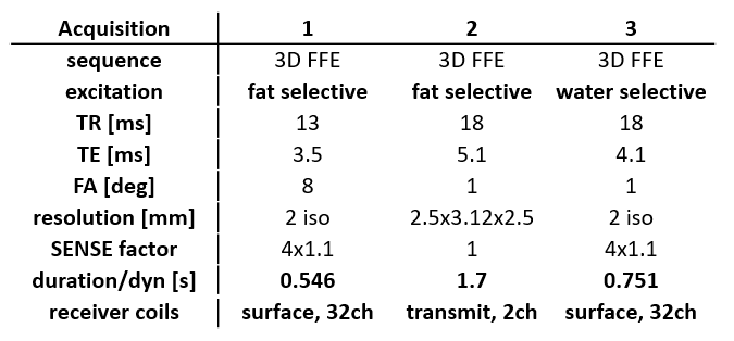
We acquired data from 4 participants at 7T MRI system (Philips, Netherlands) equipped with a 2 channel transmit, and 32 channel receive surface coils⁴. Line-scanning data acquisition used a modified 5 echoes gradient-echo sequence¹ where the phase-encoding in the direction perpendicular to the line was turned off: line resolution=250μm, TR=105ms, TE1=6ms, ∆TE=8ms, readout bandwidth=131.4 Hz/pixel, fa=16°, array size=720, line thickness=2.5mm, in-plane line width=4mm, fat suppression using SPIR. Two saturation pulses (7.76 ms pulse duration) suppressed the signal outside the line of interest. The line was positioned as perpendicular to the cortex as possible. For every scan we performed PMC, achieved by an interleaved scanning architecture (MISS, Philips) at every dynamic (i.e. every 440 timepoints = ~46s) (Figure 1). During the functional scan, the last acquired navigator volume was registered to the previous one in the series (wait=1s), and translation and rotation parameters of both the navigator and target sequence were updated in real time³. Three possible navigators were investigated (Figure 2): a highly-accelerated surface-coil-receive fat-navigator only covering the back of the head, a slower whole-head, transmit-coil-receive fat-navigator and a water-excitation navigator, aimed at reducing the amplitude of the T₁-transient. We acquired one run of functional data (6min 20s) with each scan, using a block design visual task consisting of a 20 Hz flickering checkerboard, presented for 10s ON/OFF, starting and ending with 10s baseline. We investigated 3 ways of managing the presence of gaps and T₁-transient:
1. Regressing out the T₁-transient during the general linear model (GLM) analysis (regressed)
2. Interpolating the points corresponding to the T₁-transient by substituting them with the average of the points before and after the T₁-transient (interpolated)
3. Applying a T₂* fit reconstruction to avoid T₁ effects (T₂* fit)
The timepoints of the visual task model corresponding to the time during which the navigators were acquired, were removed from the GLM. We evaluated the beta values and temporal signal to noise ratio (tSNR) along the line, to find the best acquisition and analysis strategy.

Results & Discussion

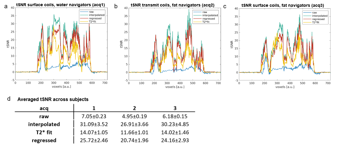
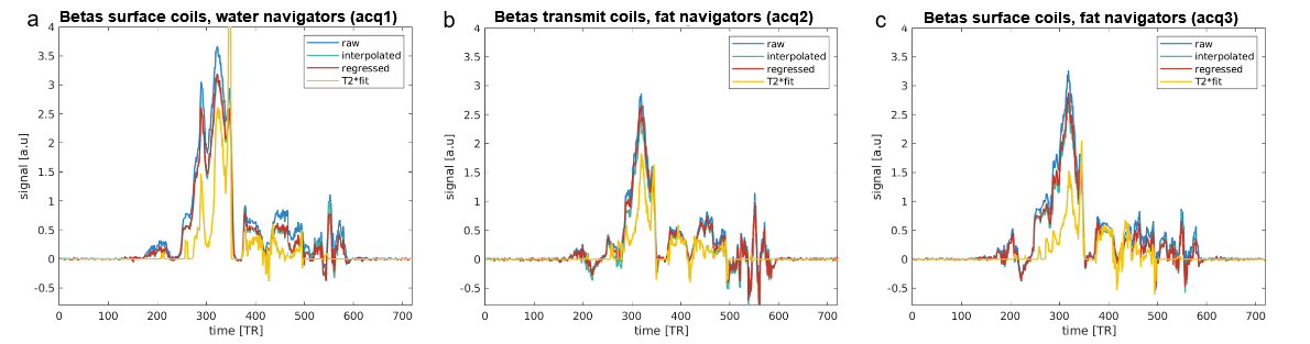
Figure 3 shows a single voxel timecourse for the three acquisitions (a, b and c), for raw data, regressed, interpolated and T²*fit. BOLD responses were visible in all timecourses, despite the T₁-transient. Notice that the shorter, more undersampled, navigators (acq 1 and 3) resulted in lower T₁-transient height. The utilization of water excitation for the navigators reduced the T₁-transient height further. For all acquisitions, the T₁-transient was much reduced after GLM-based signal regression and completely disappeared in T₂* fit data. In Figure 4, the tSNR for the interpolated data was superior to the regressed and T₂*fit data. This trend was consistent over participants (Figure 4d). The tSNR of the regressed data was reduced by remaining T₁-related instabilities, which we were not able to remove with a single-exponential regressor. The T₂* fit from our current data proved too noisy, which further reduced tSNR. Figure 5 shows the beta values for the three acquisitions (a, b and c) of a representative participant for raw data and for the three strategies of handling the presence of gap in the acquisitions and the T₁-transient. Interpolated and regressed data show similar beta values to raw data. Notice that beta values were higher in the raw data due to the presence of high signal intensities caused by the T₁-transient that corresponded with task ON blocks, while the estimation of betas is less, or not, biased when interpolated or regressed data are used. The T₂*fit data appear to suffer from increased noise, and instabilities (as apparent from the lower tSNR) which reduces the fit results.

Conclusion

We implemented prospective motion correction for line-scanning in order to prevent motion-related signal changes during line-scanning acquisitions. Overall, among the three navigators tested, the navigators acquired with water excitation and surface coils (acq 1) presented the lowest amplitude of the T₁-transient signal. The T₁-transient introduced by the navigators can be best dealt with by interpolating the affected time points. This leads to higher temporal stability (tSNR) than fitting the T₁-transient or T₂* fit-based timecourses.

Acknowledgements

This study was supported by the Royal Netherlands Academy of Arts and Sciences Research Fund 2018 (KNAW BDO/3489), the NWO TTW VIDI grant (VI.Vidi.198.016) and the Visiting Professors Program 2017 (KNAW WF/RB/3781) granted to the Spinoza Centre for Neuroimaging.