Introduction

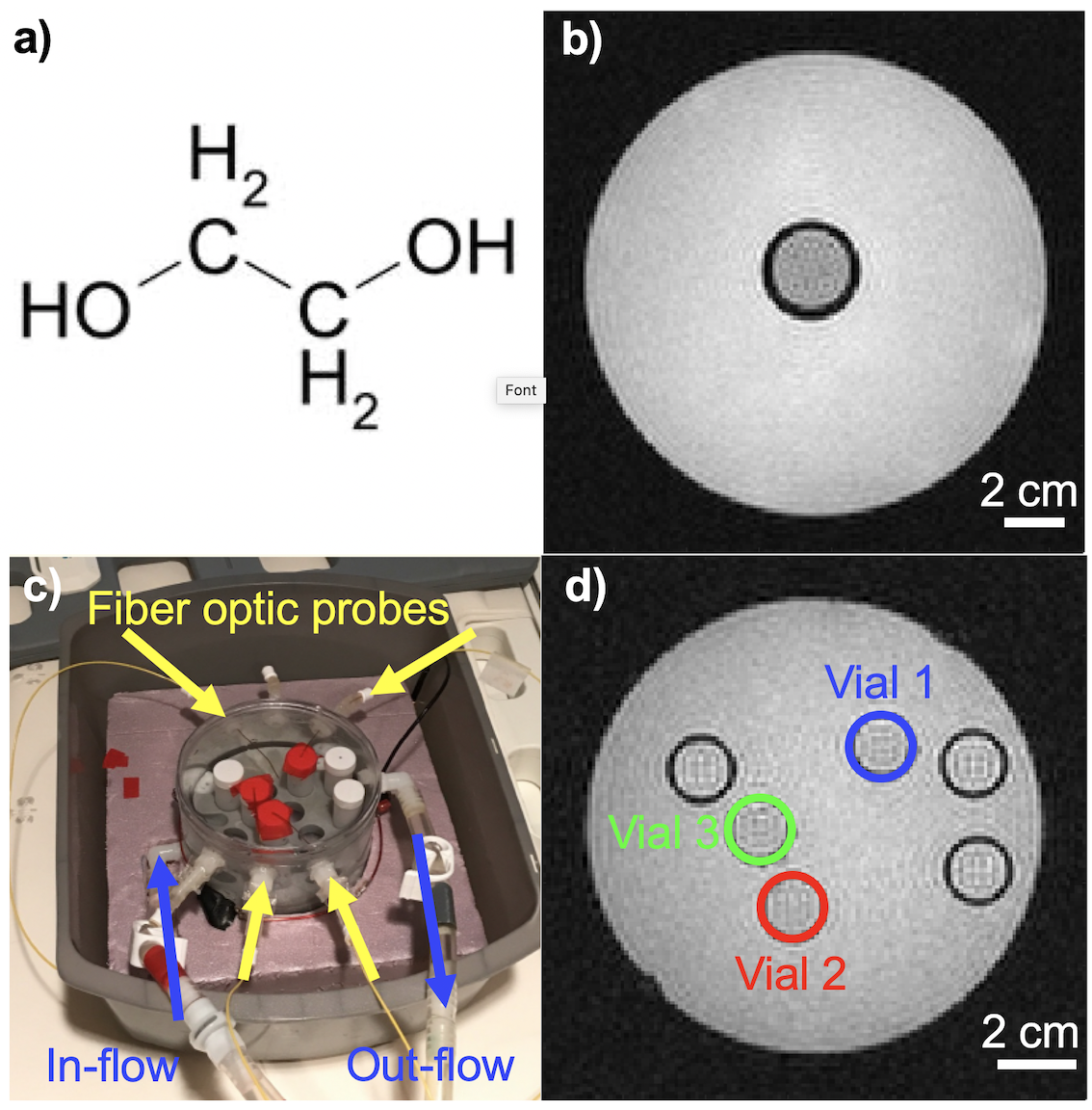
Magnetic resonance imaging (MRI) is the most commonly used medical imaging modality for non-invasive temperature measurements. However, most currently used methods, such as the phase-based proton resonance frequency shift, T1, and T2, only provide measures of temperature change.¹ Absolute temperature measurements can be performed using temperature sensitive contrast agents and spectroscopic approaches.^2,3 Temperature sensitive contrast agents change image contrast at pre-determined temperatures, and typically only provide change at one absolute temperature. Spectroscopic approaches typically have low spatial and temporal resolution. For ex vivo applications, the temperature dependent shift between the CH₂ and OH groups of Ethylene Glycol (EG), Figure 1a, has previously been used to measure absolute temperature using spectroscopic approaches.^4,5 In this work we investigate if multi-echo MRI of Ethylene Glycol can be used for high spatial and temporal resolution absolute temperature imaging for ex vivo applications. This can, e.g., be useful for absolute temperature measurements throughout phantoms used for quantitative parameter mapping (T1, T2, diffusion), which is of importance since these parameters have inherent temperature dependences.

Methods

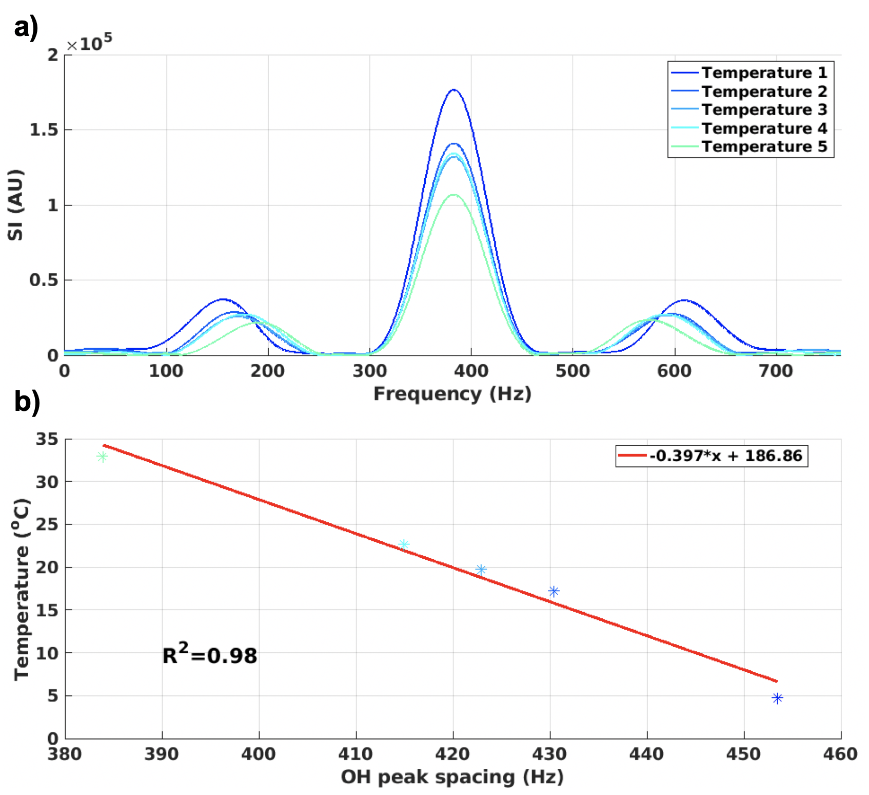
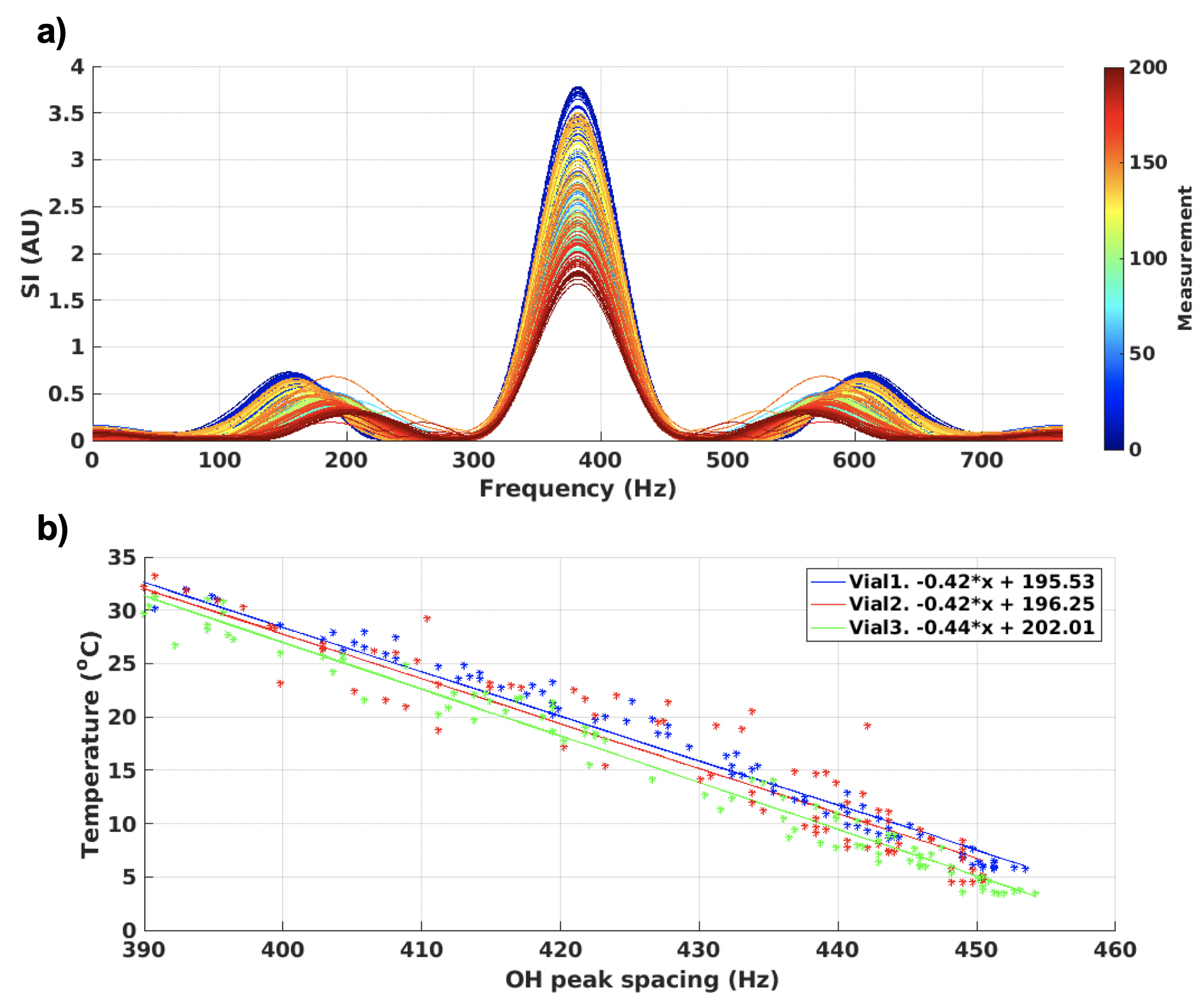
A multi-echo gradient recalled echo pulse sequence was used to acquired data at 3T (PrismaFIT, Siemens); FOV=256x256 mm, 1.33x1.33 mm, 3 mm slice, TR=31 ms, BW=1000 Hz/px, 20 echoes with TE from 2.38 to 27.46 ms, in steps of 1.32 ms (total BW=763 Hz), acquisition time 6 s. Two experiments were performed; 1) Five 2.5 cm diameter vials with EG (ThermoFisher Scientific) were placed in 15 cm diameter water baths with temperatures ranging from ~5 to 35 °C and allowed to equilibrate for at least 30 minutes. The water bath and EG vial were then scanned for five back-to-back measurements (total scan time 30 s) using the sequence noted above. 2) Three 1.5 cm diameter vials with EG were placed in a 12 cm diameter chamber which allowed flowing water to heat and cool the EG vials, Figure 1c-d. The vials were heated-cooled-heated in a range of ~5 – 50°C, while acquiring one image every 30 s (for 200 total images). The water flow was only turned on for 5-10 s after each acquisition, so the water motion slowed down for ~20 s before each subsequent acquisition to minimize motion artifacts. For all experiments, a fiber optic probe (ReFlex, Neoptix) was placed in each vial and used to measure the absolute temperature at all times. Before each experiment the probes were calibrated in an ice bath to adjust for their respective offset. Data analysis was performed in Matlab (Mathworks) and included standard image reconstruction followed by application of a Hamming window to reduce Gibb’s ringing, zero-filled interpolation to minimize partial volume effects, and taking the FFT, all applied along the echo dimension. The resulting spectra consists of a single large on-resonance CH₂ peak and two smaller OH peaks (cosine positive and negative frequency), Figures 2a and 3a. The positions of the OH peaks were located using the “findpeaks” command in Matlab, and their spacing was investigated as a function of temperature, assuming a linear relationship as previously described.^4,5 To test repeatability the temperature relationship fit from experiment 1 was applied to the data from experiment 2.

Results

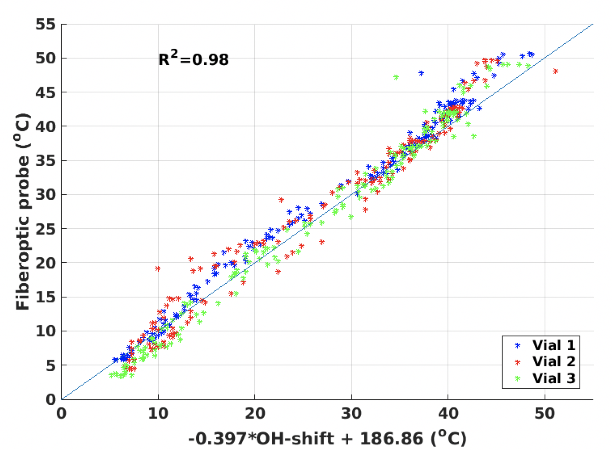
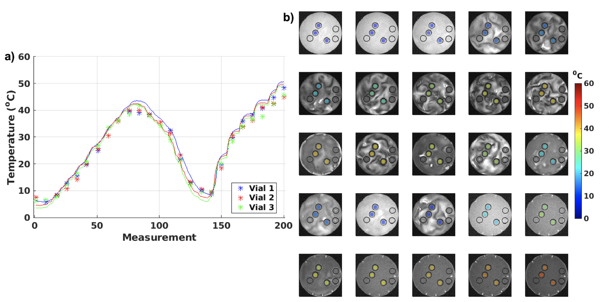
Figure 2a shows the spectra for experiment 1 for temperatures 1 – 5 (~5–35°C), and Figure 2b show temperature plotted as a function of the corresponding spacing of the OH-peaks (in Hz). A linear relationship between temperature and spacing between OH peaks of -0.397x + 186.86 was found. The spectra for measurements in one vial, for all 200 measurements from experiment 2 are shown in Figure 3a, while Figure 3b shows temperature as a function of OH peak spacing. Linear fits were performed for the data from each vial and the slope and y-intercept were slightly higher than that found in experiment 1 (0.42-0.44°/Hz and 196-202°, respectively). Despite this, Figure 4 shows that if the fit from experiment 1 (i.e., -0.397x + 186.86) were applied to the data from experiment 2 to convert OH peak spacing to absolute temperature, good agreement with probe measurements were achieved (R²=0.98). The root-mean-square error between the probe and MRI measurements for all three vials was 2.3°C. Figure 5 shows absolute temperatures for the three vials overlaid on magnitude images, again using the temperature relationship from experiment 1 applied to the data from experiment 2 to convert OH peak spacing to absolute temperature. Despite motion artifacts in the water bath the temperature measurements are flat across each vial.

Discussion and Conclusions

Both spectroscopic imaging experiments performed in this work demonstrated that the OH peak spacing of EG changes linearly with temperature, as previously shown with spectroscopic methods. The results were repeatable and the fit from one experiment could accurately (~2°C) be used to measure absolute temperatures in a second experiment. It is expected that the accuracy can be further improved if a no-flow phantom is used and by acquiring multiple signal (i.e., image) averages (as is commonly done in spectroscopy).This work shows that MRI of EG can be used to achieve high temporal and spatial resolution absolute temperature measurements over experimentally relevant fields of view. This can be useful for spatial temperature measurements in phantoms used for quantitative parameter mapping.

Acknowledgements

This work was supported by NIH grants R01EB028316, R03EB029204, S10OD026788 and S10OD018482.