Introduction

The Biot-Savart-law is an easy-to-implement method providing a good approximation for a variety of field computational problems in MRI^1-2. This method has been used to compute sensitivity profiles of surface coils or the spatially dependent magnetic fields of gradient coils^3-5. More complex designs such as birdcage coils or RF-shields can also be evaluated with this method^6-8. The achieved successes are the reason why the Biot-Savarat-law has become a fundamental tool and thinking aid for RF-engineers. However, due to the trend towards higher field strengths, the Biot-Savart-law has become less applicable as the results obtained no longer match the field measurements. In this work, we aim to demonstrate that the less-known time-generalized Biot-Savart law can be used to compute $$$B_1^+\;$$$and $$$B_1^-\;$$$fields of surface coils for different frequencies. Furthermore, we investigate whether the time-generalized form can be used to synthesize $$$B_1$$$-fields of coil arrays in CP-mode.

Methods

Definitions: The time-generalized Biot-Savart-law (also referred as Jefimenko's equation for the mangetic field) is given by^9-14:

$$\mathbf{B}(\mathbf{r},t)=\frac{\mu_0}{4\pi}\int_C\left[\frac{I(\mathbf{r'},t_r)\mathbf{dr'}\times(\mathbf{r'}-\mathbf{r})}{|\mathbf{r'}-\mathbf{r}|^3}+\frac{\dot{I}(\mathbf{r'},t_r)\mathbf{dr'}\times(\mathbf{r'}-\mathbf{r})}{c_m|\mathbf{r'}-\mathbf{r}|^2}\right].\qquad[1]$$

Here is $$$I(\mathbf{r'},t_r)\mathbf{dr'}$$$ the time varying current element at $$$\mathbf{r'}$$$, $$$\dot{I}(\mathbf{r'},t_r)\mathbf{dr'}$$$ the time derivative of the current element, $$$t_r=t-|\mathbf{r'}-\mathbf{r}|/c_m$$$ the retarded time and $$$c_m=c_0/\sqrt{\epsilon_r}$$$ the speed of light. If we assume a harmonic time-dependence, Eq.1 reads as follows¹⁵:

$$\mathbf{B}(\mathbf{r},\varphi)=\frac{\mu_0}{4\pi}\int_CI(\mathbf{r'})\mathbf{dr'}\times(\mathbf{r'}-\mathbf{r})\exp\left[j(\frac{\omega|\mathbf{r'}-\mathbf{r}|}{c_m}+\varphi)\right]\left[\frac{1}{|\mathbf{r'}-\mathbf{r}|^3}+\frac{j\omega}{c_m|\mathbf{r'}-\mathbf{r}|^2}\right].\qquad[2]$$

With this equation, $$$B_1^+$$$ and $$$B_1^-$$$ can be calculated with the well known relationships¹⁶:

$$B_1^+=\frac{1}{2}(B_x+jB_y).\qquad[3]$$$$B_1^-=\frac{1}{2}(B_x-jB_y)^*.\qquad[4]$$

To calculate the current distribution $$$I(\mathbf{r'})=I(\phi)$$$ of a circular surface coil, a Fourier-expansion can be used¹⁷:

$$I(\phi)=\sum_{n=-\infty}^{\infty}I_n\exp(jn\phi).\qquad[5]$$

The current coefficients $$$I_n$$$ are calculated as follows:

$$I_n=j\beta_0V\pi^{-1}\xi_0^{-1}\left[\frac{1}{2}\beta_0^2b^2(k_{n+1}+k_{n-1})-n^2k_n\right]^{-1},\qquad[6]$$

$$k_0=(\pi b)^{-1}\left[\ln(8b/a)-\frac{1}{2}\pi\int_{0}^{2\beta_0b}dx\left[\Omega_0(x)- jJ_0(x)\right]\right],\qquad[7]$$

$$k_n=k_{-n}=(\pi b)^{-1}\left[K_0(na/b)I_0(na/b)+\left[\ln(4n)+\gamma-2\sum_{m=0}^{n-1}(2m+1)^{-1}\right]-\frac{1}{2\pi}\int_{0}^{2\beta_0 b}dx\left[\Omega_{2n}(x)-jJ_{2n}(x)\right]\right].\qquad[8]$$

Here are $$$a$$$ and $$$b\;$$$the wire and loop radius, $$$V\;$$$the excitation-voltage, $$$\gamma=0.57722\;$$$Euler's constant, $$$\beta_0=2\pi/\lambda=\omega/c$$$ the electric-length, $$$\xi_0=\sqrt{\mu_0/\epsilon_0}\;$$$the free space wave-impedance, $$$\Omega_n\;$$$the Lommel-Weber-function of order $$$n$$$, $$$J_n\;$$$the Bessel-function of the first kind and order $$$n\;$$$and finaly$$$\;K_0\;$$$and$$$\;I_0\;$$$are the modified Bessel-functions of the first and second kinds and order zero.

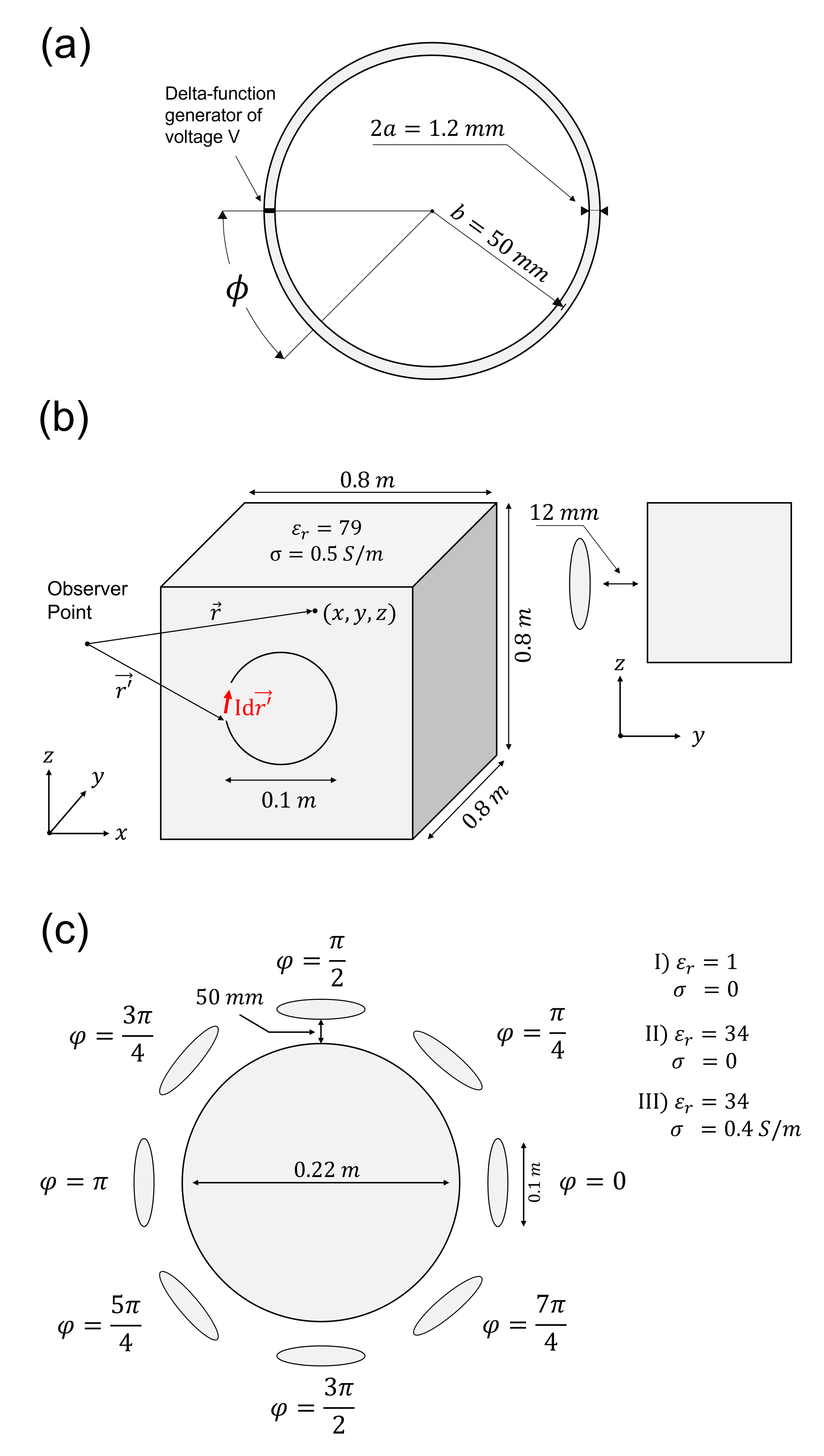
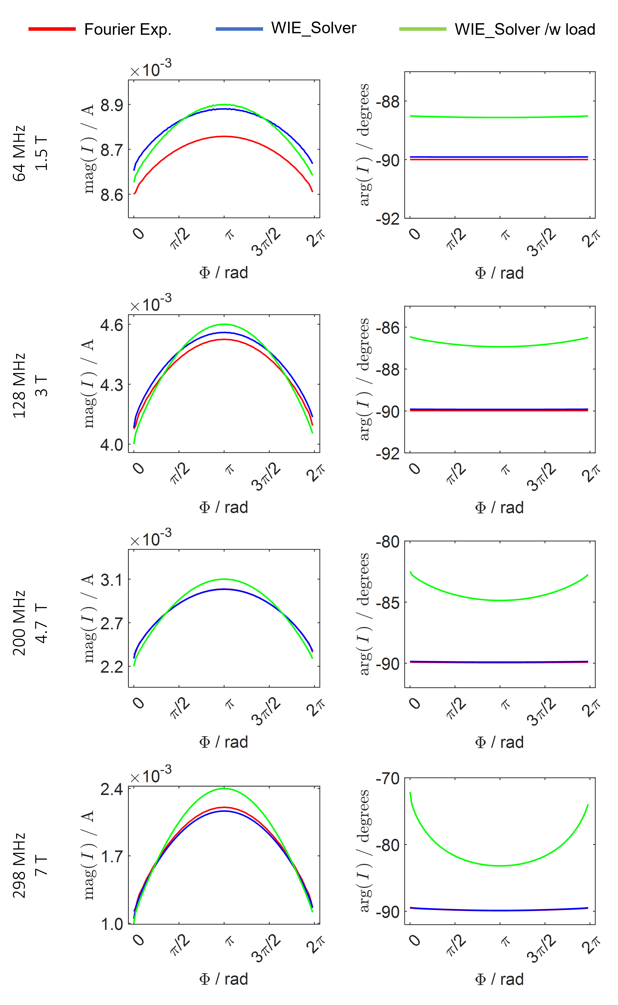
Simulations: (i) Current-computation: we calculated $$$I(\mathbf{r'})\;$$$according to the approach presented above. However, as this approach does not take loading effects into account, we computed the current for a circular loop (Fig.1a) for the frequencies$$$\;64,\,128,\,200\;$$$and$$$\;298\,MHz\;$$$and compared the results with the current obtained when using the WIE_Solver¹⁸ from the MARIE-package^19-20, for the loaded and unloaded case respectively $$$(\epsilon_r = 79,\sigma = 0.5\,S/m)$$$.

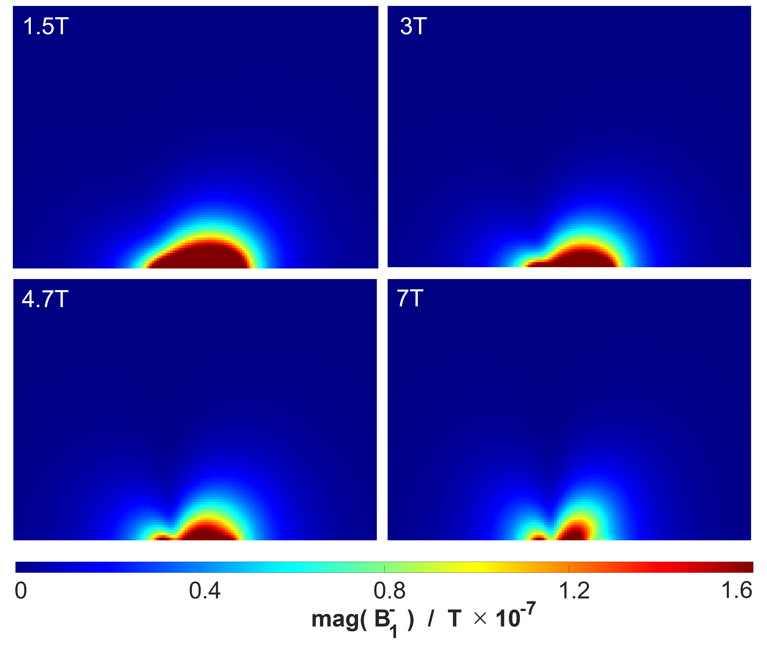
(ii) $$$B_1^-$$$-computation: we calculated the $$$B_1^-$$$-field for the same circular surface coil placed on a cuboid load (Fig.1b) by solving Eq.2 for the frequencies$$$\;64,\,128,\,200\;$$$and$$$\;298\,MHz$$$. To account for $$$\sigma$$$-damping we extended Eq.2 with $$$exp(-\alpha |\mathbf{r'} - \mathbf{r}|)$$$. The attenuation-constant $$$\alpha\;$$$is given by:
$$\alpha=\omega\sqrt{\frac{\mu\epsilon}{2}\left[\sqrt{1+\left[\frac{\sigma}{\omega\epsilon}\right]^2}-1\right]}.\qquad[9]$$
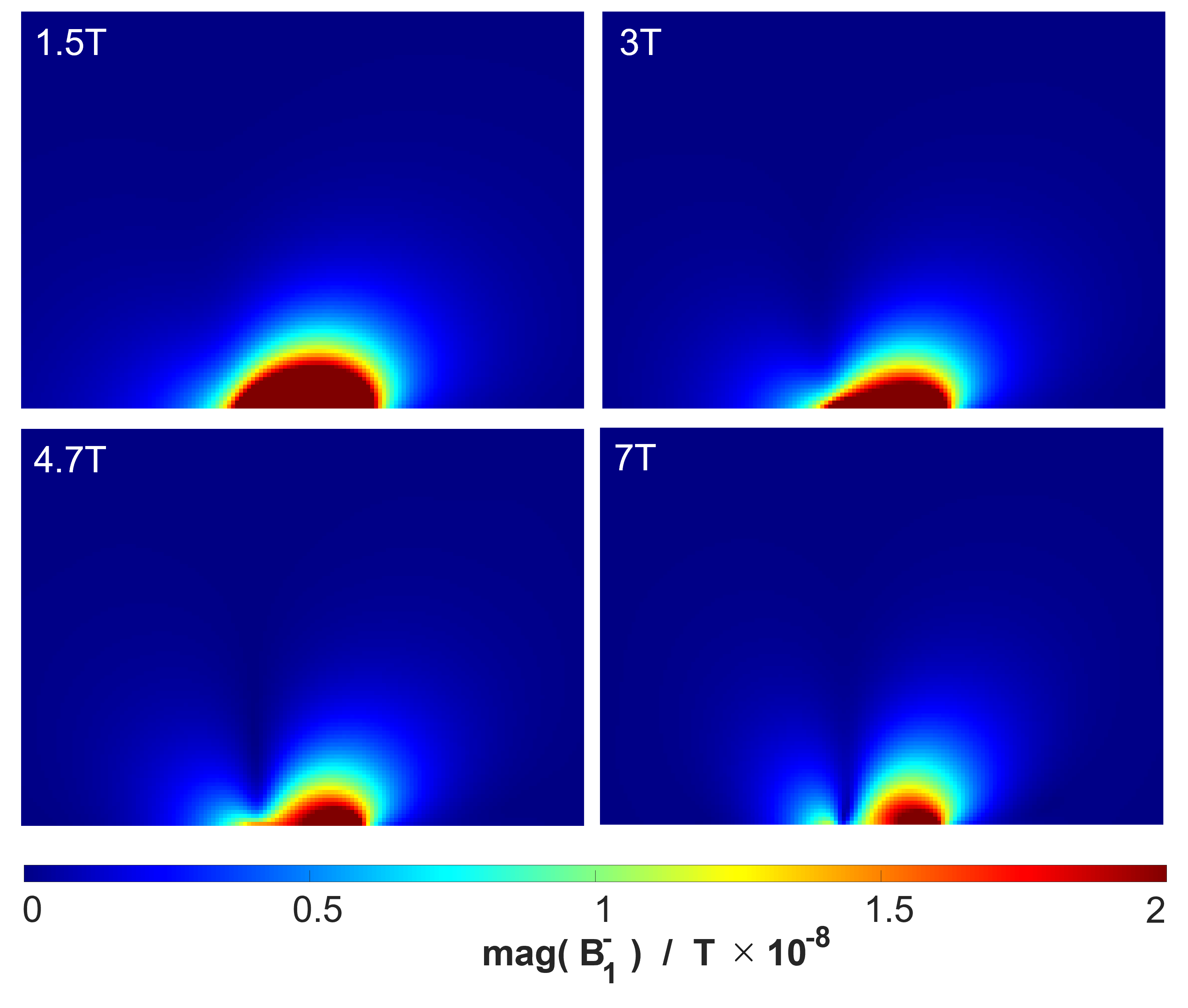
We compared the results against the $$$B_1^-$$$-fields obtained from the MARIE package. Since the time-generalized Biot-Savart-law does not account for wave reflections, a large loading volume was chosen for fair comparison. It should be noted that the magnitudes of $$$B_1^+\;$$$and $$$B_1^-$$$ are mirror pairs.

(iii)$$$B_1$$$-computation: we computed the $$$B_1$$$-field for the coil array shown in Fig.1c when the array is operated in CP mode at $$$298\,$$$MHz, respectively for:

• (I)$$$\,\,\epsilon_r=1\;$$$and$$$\;\sigma=0$$$,
• (II)$$$\,\,\epsilon_r=34\;$$$and$$$\;\sigma=0$$$,
• (III)$$$\,\,\epsilon_r=34\;$$$and$$$\;\sigma=0.4\,S/m$$$.

Therefore, we solved Eq.2 for each coil $$$n$$$ and phase $$$\varphi=(n-1)2\pi/8$$$ and then extracted the real part of the complex field. Finally, the $$$B_1$$$-field was formed by superposition.

Results

(i) The mean deviation between the magnitude of the currents obtained from the Fourier expansion and the WIE_solver was $$$0.9\,\%$$$ and $$$3.8\,\%$$$ for the unloaded and loaded case, respectively (Fig.2). The mean deviation between the phase of the currents turned out to be$$$\;0.1\,\%$$$ and $$$8.3\,\%$$$ for the unloaded and loaded case.

(ii) The$$$\;B_1^-$$$-fields calculated using the time-generalized Biot-Savart-law (Fig.3) shows that with increasing frequency the fields become more structured due to shorter wavelength effects. Comparison of the Biot-Savart fields with the results of MARIE (Fig.4) shows qualitatively a high level of agreement. Note, that the peak value of the Biot-Savart $$$B_1^-$$$-field is larger by an order of magnitude.

(iii) As expected, the computed $$$B_1$$$-fields (Fig.5) of the investigated coil array show a homogeneous circularly polarized field when the array is unloaded $$$(\epsilon_r=1$$$,$$$\;\sigma=0$$$). For the lossless loaded case $$$(\epsilon_r=34$$$,$$$\;\sigma=0)\;$$$a central brightening was observed. For the lossy loaded case $$$(\epsilon_r=34$$$,$$$\;\sigma = 0.4\,S/m)$$$ the central brightening effect was attenuated.

Discussion

We showed that the time-generalised Biot-Savart-law is an easy-to-implement method for$$$\;B_1^+\;$$$and$$$\;B_1^-$$$-field calculations. The results agree well with those obtained from the full-wave solver MARIE. Furthermore, we showed that the presented method is well-suited for$$$\;B_1\;$$$evaluations of array coils in CP-mode. It should be mentioned, however, that we only obtained well-matched results, because we have chosen a load geometry with low reflection. For more complex loading geometries, the deviation from a full-wave solver may be larger because the reflected components are not taken into account. The discrepancy by an order of magnitude between the fields obtained by the time-generalized Biot-Savart approach and the MARIE solver could be attributed to the absence of any reflections at the load boundaries.
However, this work has shown that several field properties of RF coils can be predicted using the time-generalized Biot-Savart law. In future studies, we will further investigate whether this approach can be extended to account for wave reflections. This would allow to evaluat coil arrays for SNR performance and acceleration capabilities.

Conclusion

The presented method for$$$\;B_1\;$$$field calculations using the time-generalized Biot-Savart-law is a suitable alternative to computationally demanding full-wave solvers, when wave reflections are negligible. Further research will be needed to include reflection phenomena.

Acknowledgements

References

1. Wright, Steven M., and Lawrence L. Wald. "Theory and application of array coils in MR spectroscopy." NMR in Biomedicine: An International Journal Devoted to the Development and Application of Magnetic Resonance In Vivo 10.8 (1997): 394-410.
2. Wright, Steven M., Richard L. Magin, and James R. Kelton. "Arrays of mutually coupled receiver coils: theory and application." Magnetic resonance in medicine 17.1 (1991): 252-268.
3. Wang, Jianmin, Arne Reykowski, and Johannes Dickas. "Calculation of the signal-to-noise ratio for simple surface coils and arrays of coils [magnetic resonance imaging]." IEEE transactions on biomedical engineering 42.9 (1995): 908-917.
4. Roemer, Peter B., et al. "The NMR phased array." Magnetic resonance in medicine 16.2 (1990): 192-225.
5. Liu, Wentao, et al. "Target-field method for MRI biplanar gradient coil design." Journal of Physics D: Applied Physics 40.15 (2007): 4418.
6. Giovannetti, Giulio, et al. "A fast and accurate simulator for the design of birdcage coils in MRI." Magnetic Resonance Materials in Physics, Biology and Medicine 15.1 (2002): 36-44.
7. Jin, Jianming, Gary Shen, and Thomas Perkins. "On the field inhomogeneity of a birdcage coil." Magnetic resonance in medicine 32.3 (1994): 418-422.
8. Wright, S. M., and J. R. Porter. "An enhanced Biot-Savart law modeling technique for RF coils with unknown current distributions and shields." Proceedings of the 2nd Annual Meeting of the Society of Magnetic Resonance. Abstr. 1994.
9. Jefimenko, Oleg D. Electricity and magnetism: an introduction to the theory of electric and magnetic fields. Electret Scientific Company, 1989.
10. Jefimenko, Oleg D. "Solutions of Maxwell’s equations for electric and magnetic fields in arbitrary media." American journal of physics 60.10 (1992): 899-902.
11. Griffiths, David J., and Mark A. Heald. "Time‐dependent generalizations of the Biot–Savart and Coulomb laws." American Journal of Physics 59.2 (1991): 111-117.
12. Griffiths, David J. "Introduction to Electrodynamics Fourth Edition", Cambridge University Press, (2017).
13. Jackson, John D., "Classical Electrodynamics Third Edition",
Wiley, (1998).
14. Freeman, Richard R., James A. King, and Gregory P. Lafyatis. "Electromagnetic radiation", Oxford University Press, (2019).
15. Tokaya, Janot P., et al. "MRI‐based transfer function determination through the transfer matrix by jointly fitting the incident and scattered field." Magnetic resonance in medicine 83.3 (2020): 1081-1095.
16. Hoult, D. I. "The principle of reciprocity in signal strength calculations—a mathematical guide." Concepts in Magnetic Resonance: An Educational Journal 12.4 (2000): 173-187.
17. Wu, Tai Tsun. "Theory of the thin circular loop antenna." Journal of Mathematical Physics 3.6 (1962): 1301-1304.
18. Harrington, Roger F. "Matrix methods for field problems." Proceedings of the IEEE 55.2 (1967): 136-149.
19. Polimeridis, Athanasios G., et al. "Stable FFT-JVIE solvers for fast analysis of highly inhomogeneous dielectric objects." Journal of Computational Physics 269 (2014): 280-296.
20. Villena, Jorge Fernandez, et al. "MARIE–a MATLAB-based open source
software for the fast electromagnetic analysis of MRI systems." Proceedings of the 23rd Annual Meeting of ISMRM, Toronto, Canada. 2015.