Introduction

Chemical Exchange Saturation Transfer (CEST) MRI has proven its clinical value in numerous opportunities¹. One drawback of CEST is its long acquisition time, making the translation into clinical routine challenging. Therefore, snapshot CEST² was introduced. Snapshot CEST acquires the whole 3D k-space after just one saturation block, thereby reducing the measurement time to an absolute minimum. This comes at the cost, of only being able to acquire a limited amount of k-space lines after one CEST saturation. Which ultimately translates into a reduced coverage. Snapshot CEST employs in its original form a gradient echo (GRE) readout (RO). Lately, to increase the coverage again, it was combined with an Echo-Planar-Imaging (EPI) RO, which showed promising results in the brain³. EPI, on the other hand, has the disadvantage of being sensitive to B0-related artefacts, which hinders its application in other body regions than the brain. Therefore, we suggest to still use a GRE RO, but combine it with Compressed Sensing (CS). Thereby, the number of lines needed to be acquired can be kept the same, while increasing the coverage without running into distortions or signal dropout artefacts, as in EPI. At last, the offset number plays a significant role in the overall measurement time and was therefore optimised as well.

Methods

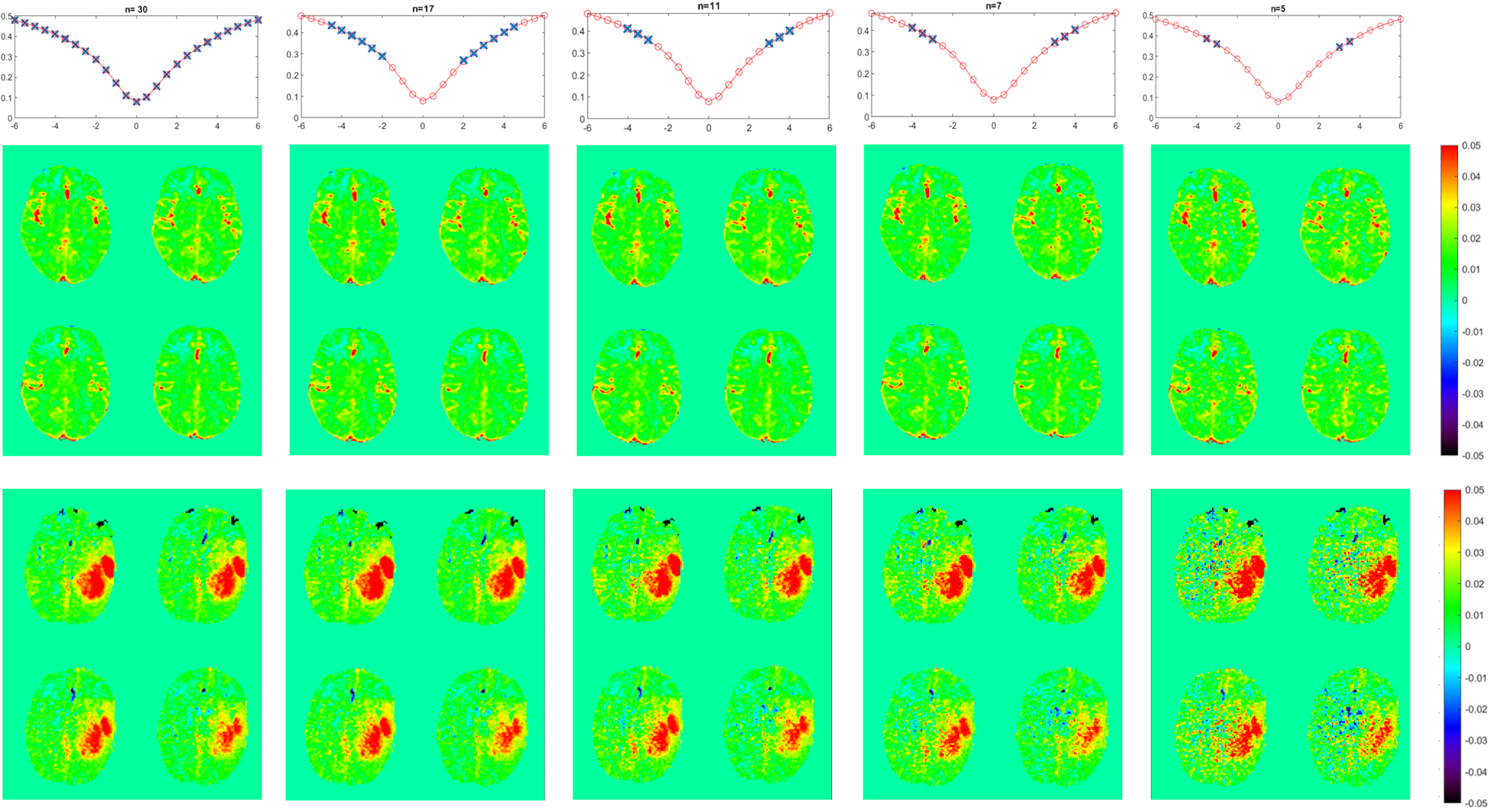
Images were obtained from healthy volunteers and 2 patients under approval of the local ethics committee. Scanning was performed on a 3T MAGNETOM Prisma MRI scanner (Siemens Healthcare, Erlangen, Germany) in combination with a 64ch head coil.
To generate a suitable ground truth 30 offsets distributed as shown in figure 1 were acquired. Retrospectively offsets were eliminated from that data set and Amide Proton Transfer-weighted (APTw) CEST maps were calculated. B0 correction was performed via spline fitting over the whole acquired points.
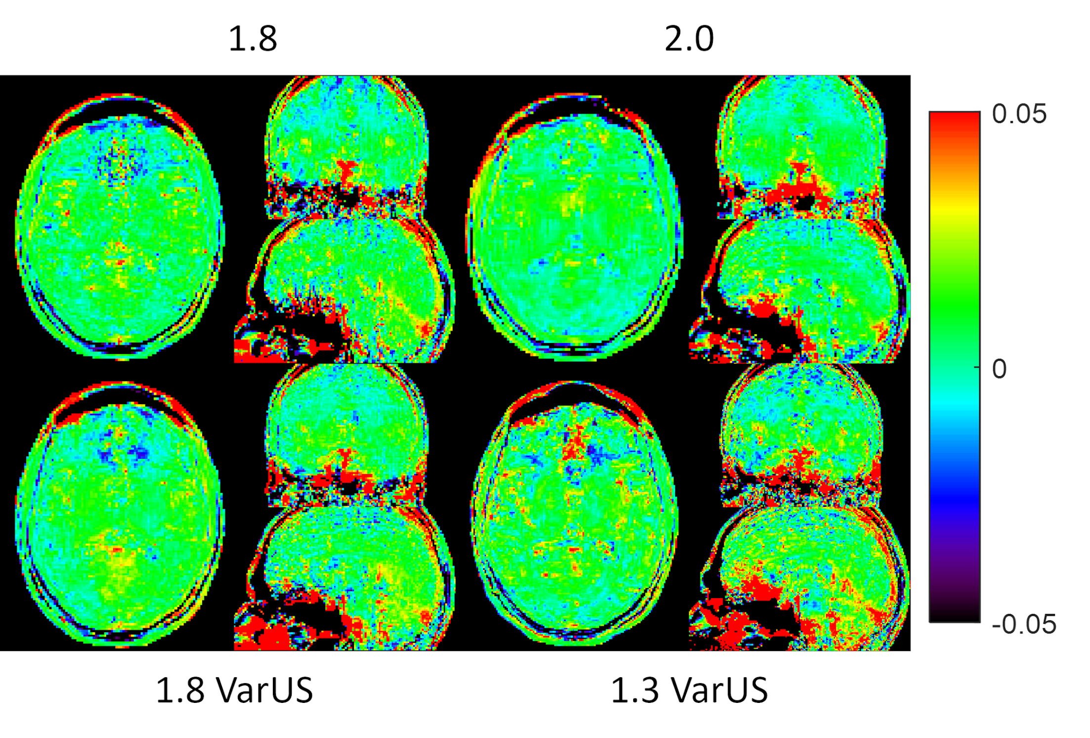
An L1 regularized, fully coupled CS reconstruction was implemented based upon a sparse incoherent spatio-temporal Poisson disk undersampling, as described in reference 4. The reconstruction itself was running online on the scanner hardware. 5 different schemes were tested: 1) the acceleration factor was kept the same as in the standard slab-selective case⁵. 2) The acceleration factor was increased to 8.66 to enable a whole brain 2 mm isotropic acquisition. 3) The acceleration factor was further increased to 10.98 to enable a 1.8 mm isotropic whole brain acquisition. 4) The undersampling mask was varied (VarUS) for the 1.8 mm isotropic protocol and regularisation along the offset dimension was introduced. 5) To test the limit of the current method, the acceleration factor was further increased to 20.65 to enable a 1.3 mm whole brain protocol. In this case, the undersampling mask was varied as well with regularisation along the offset domain. Imaging parameters can be found in table 1, the CEST preparation follows the Pulseq-CEST standard^6,7.
APTw CEST maps were generated on the scanner, using a second-degree polynomial fitting for B0 correction. B0 field maps were acquired automatically before and took 21 seconds.
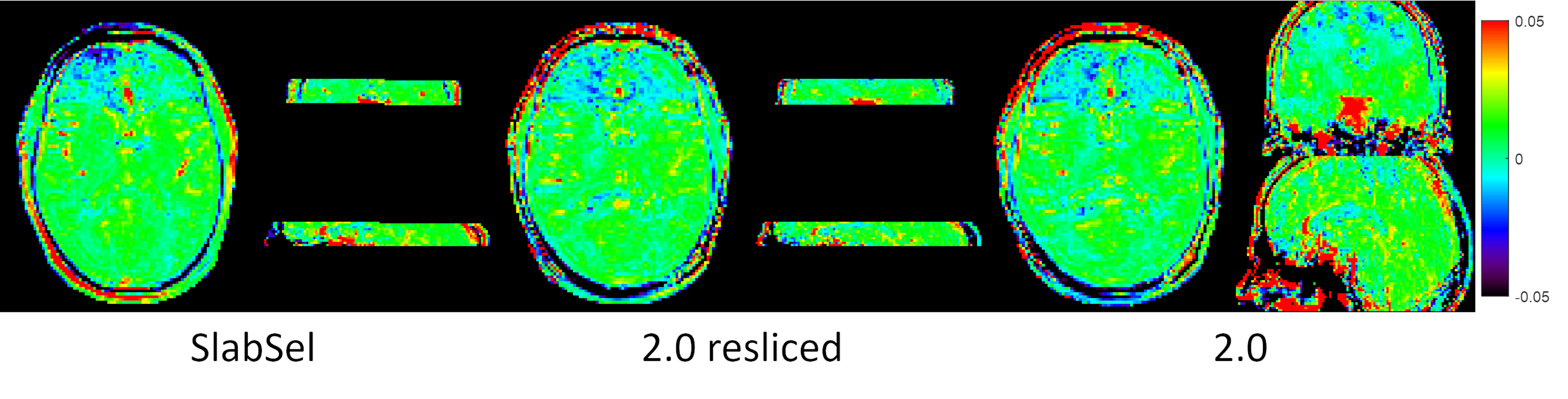
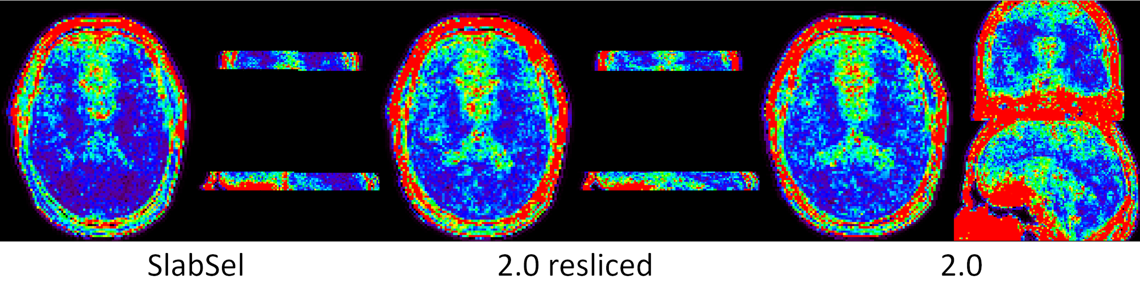
Standard Deviation maps (STD) were calculated by acquiring the APTw contrast (using the 11-point scheme depicted in figure 1) 9 times, once for the slab selective protocol and once for the whole brain 2 mm isotropic protocol. STD was calculated by first registering and reslicing all reconstructed APTw maps onto the first offset of the slab selective acquisition using SPM.

Results

In figure 1 can be seen that no loss of contrast occurs, when reducing the offset number to 11. Figure 2 shows the comparison between the slab-selective protocol (case 1 from above) and the 2 mm isotropic whole brain protocol (case 2). No significant difference can be seen. However, the standard deviation, as seen in the maps in figure 3 is about 16% lower for the slab selective protocol. Figure 4 shows the reconstructed APTw maps of cases 2 to 5, showing that a 1.3 mm isotropic whole brain acquisition is possible. Varying the undersampling mask and regularizing along the offset dimension apparently increases the Contrast-to-Noise-Ratio (CNR) in the APTw maps.

Discussion

It was shown that whole-brain 1.3 mm isotropic snapshot APTw CEST acquisitions are possible. Whole-brain acquisitions come with a higher acceleration factor and therefore a penalty in the stability, as seen in the STD maps. However, it is not clear what stability is needed in a clinical environment, where this moderate loss might be readily traded off for a whole-brain coverage in combination with short scan times. Ultimately, the APTw CEST maps look promising, even for the 1.3 mm isotropic acquisition. In the future we will be testing this approach in a tumour patient.

Conclusion

Fast whole-brain APTw CEST is possible and can be readily applied in the clinic, by using an online reconstruction and inline acquisition of field maps. This approach can be extended to other body regions and will be considered in the future. Future work will also encompass to bring this approach to 7T, where typically an even higher number of offsets is acquired.

Acknowledgements

No acknowledgement found.