2080
Principal Component selections and filtering by spatial information criteria for multi-acquisition CEST MRI denoising1Department of Research & Innovation, Olea Medical, La Ciotat, France, 2Institute of Biostructures and Bioimaging (IBB), National Research Council of Italy (CNR), Torino, Italy, 3Lysholm Department of Neuroradiology,, University College of London Hospitals NHS Foundation Trust, London, United Kingdom, 4Institute of Neurology UCL, London, United Kingdom, 5Department of Neuroradiology, University Clinic Erlangen, Friedrich-Alexander Universität Erlangen-Nürnberg (FAU), Erlangen, Germany
Synopsis
This work provides a new denoising methodology for multi-acquisition magnetic resonance images (MRI) based on principal components analysis (PCA). We are proposing a new principal component selection criterion that identifies spatial information in the extracted component coefficients, leading to a better preservation of anatomical structures and pathological information. In addition, our adaptive filtering step allows us to further denoise the MRI data, rejecting persistent spatial noise from the extracted component coefficients. In our investigations the proposed method outperformed the eigenvalue based selection criteria on Amide Proton Transfer weighted CEST data.
Introduction
Principal Component Analysis (PCA) is a non-parametric technique originally designed to reduce the dimensionality of a given dataset, while retaining the essence of the data1,2. It extracts a new set of variables, called Principal Components (PCs) which are ordered based on the variability of the original data each component explains, i.e. their associated eigenvalues.PCA has been successfully used for denoising purposes in multi-acquisition MRI, usually reconstructing the original dataset selecting the signal-related components and rejecting noise-related components. For example, in3, three eigenvalues-based methods are presented (Malinowski, Nelson and Median criteria) and thereafter investigated for their applicability to denoising of in vivo Chemical Exchange Saturation Transfer (CEST) MRI data4.
Other methods exist5,6 but many rely on the eigenvalues associated with the extracted principal components for the selection of the signal-related components. However, such methods risk discarding anatomical structures and pathological information hidden in the noise of the extracted components, especially if those areas are small, as eigenvalues measures blindly the variance of components regardless if it is noise or relevant clinical information.
A Z-Spectrum for a given voxel in the CEST data can be expressed as:
$$\mathbf{Z_i}=\overline{z_{i}}+\sum_j\alpha_{ ij}\mathbf{v_j}$$
where $$$\overline{z_{i}}$$$ is the mean value of the Z-Spectrum, $$$\mathbf{v_j}$$$ is a principal component and $$$\alpha_{ ij}$$$ is the coefficient of $$$\mathbf{v_j}$$$ of voxel $$$i$$$.
Collecting all coefficients $$$\omega_{ij}$$$ of a component $$$j$$$ in the same order of the Z-Spectra in the CEST acquisitions, we obtain the PC related image (or volume) of the $$$j^{th}$$$ component (see Figure1).
Methods
Technical Solution:Our proposed method, called Component Analysis based on Standard-deviation Attenuation (CASA) criterion is based on the decrease of the variance of a PC related image after a smoothing filter is applied on it, as detailed in the following steps (see Figure2):
1) PCA is performed to obtain the PC related images. The standard deviation of the voxels of the full image or within a segmented region (for example excluding background voxels) is computed for each of the $$$N$$$ PC related images to form the vector $$$\sigma^a=[\sigma^a_{1},\sigma^a_{2},\sigma^a_{3},…\sigma^a_{N}]$$$. Then a Gaussian smoothing filter of a factor $$$\Sigma$$$ is applied to each component and standard deviation is recomputed on the smoothed PC related images to obtain $$$\sigma^b=[\sigma^b_{1},\sigma^b_{2},\sigma^b_{3},…\sigma^b_{N}]$$$, where $$$\sigma^a_{i}>\sigma^b_{i}$$$. The rate of decrease of standard deviation is then computed, for each component, as $$$\sigma^r =(\sigma^a -\sigma^b) / \sigma^a$$$, where $$$0<\sigma^r_{i}<1$$$, $$$\forall i$$$. Components whose $$$\sigma^r_{i}$$$ rate is on the plateau of the curve are rejected (see Figure2).
2) Before the signal reconstruction a smoothing filter or denoising method can be applied on the retained PCs (PC related images). The strength of the applied filter is proportional to the amount of information that the $$$i^{th}$$$ component carries expressed in $$$\sigma^r_{i}$$$, as $$$w^r_{i}=(\sigma^r_{i}-\sigma^r_{1})/(\sigma^r_{plateau}-\sigma^r_{1})$$$ (see Figure2). This allows to optimize the filtering method based on the amount of noise and information present in each component.
3) The retained component coefficients are projected back in the original space and used for the denoised data reconstruction.
Carrying out only the first and third step, we call the method “CASA basic”, and “CASA advanced” when all three steps are applied.
Patient data acquisition and postprocessing:
Imaging clinical data on a glioma patient were acquired on a 3T whole-body MRI system (MAGNETOM Prisma; Siemens Healthcare, Erlangen, Germany) with a 64-channel Head/Neck coil. A 3D snapshot-GRE CEST protocol7 (MPI03) was used to acquire WASAB18 and Amide Proton Transfer weighted4 (APTw) data with parameter details listed in Figure3. Data were motion corrected with SimpleElastix9. Olea Sphere 3.0 (Olea Medical, La Ciotat, France) was used to compute B0/rB1 map from WASAB1 and correct the APTw-Z-Spectra.
Synthesized data:
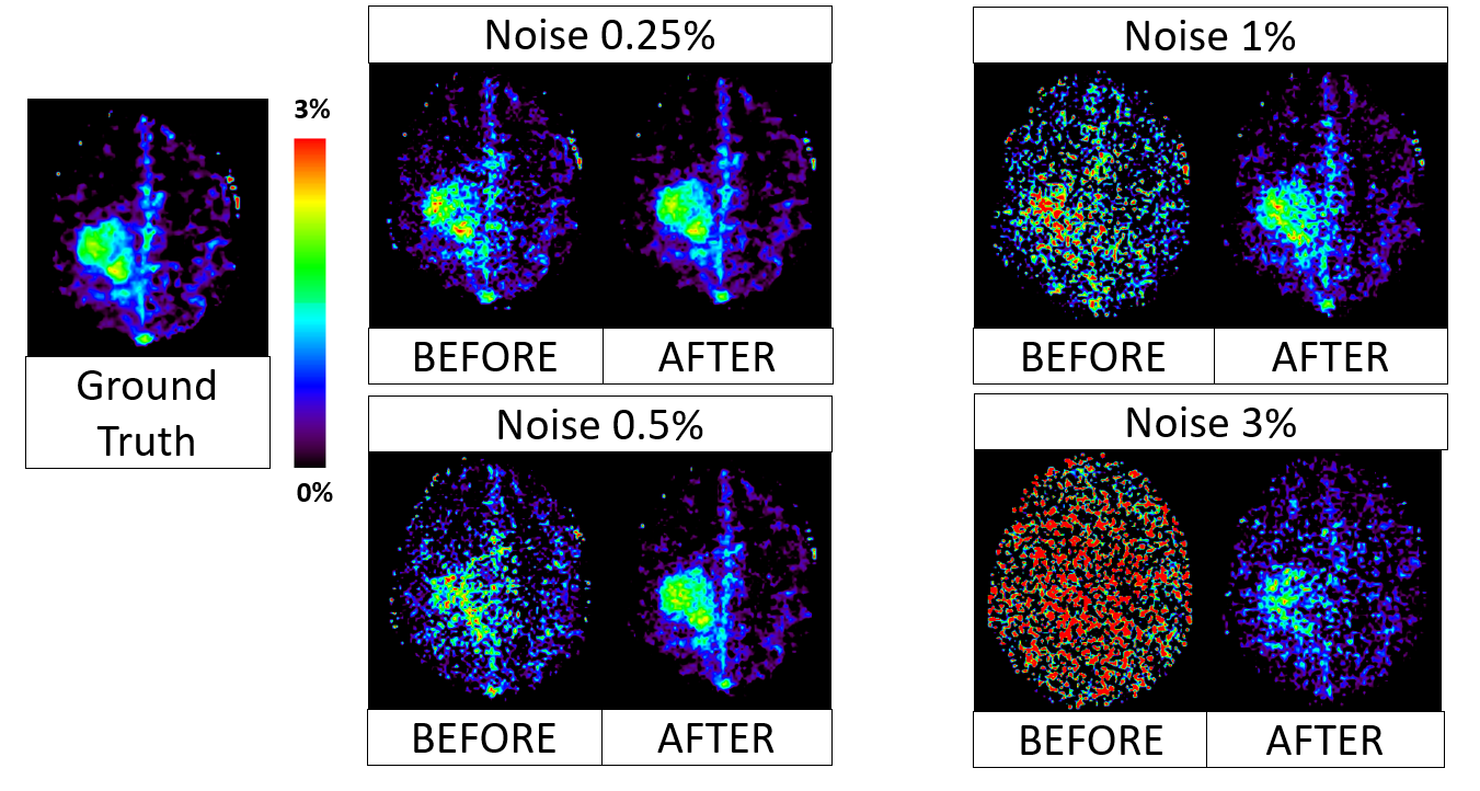
A simulated brain phantom was generated starting from the clinical APTw dataset with its same 3D resolution. The Z-Spectra were fitted with the Bloch-McConnel equations modified to include the exchange terms with a five pools model10,11, using MATLAB (parameters in Figure3). The phantom (ground truth) Z-Spectrum volumes were computed at 25 equally-spaced offsets from -6ppm to 6ppm (step=0.5ppm).
The phantom was corrupted by several percentage levels of Rician noise (0.25%,0.5%,1%,3% of the maximum intensity for each Z-Spectra) in frequency domain. The phantom data were PCA denoised using both CASA methods, Malinowski, Nelson and Median selection criteria. MTRasym12 (at 3.5ppm) maps were computed on the ground truth and on various denoised data. These maps were used for comparison.
Results
Data quality analysis using Peak signal-to-noise ratio (PSNR), Structural Similarity Index (SSIM), Correlation and Mean Square Error (MSE) have been used to evaluate the goodness of the various denoising methods.The results in Figure4 shows that for all noise levels "advanced CASA" metric leads to the best results (highest PSNR/SSIM/Correlation and Lowest MSE). Figure5 shows the MTRasym maps of ground truth, data corrupted by various noise levels, and after PCA denoising with "advanced CASA" criterion.
Discussion and Conclusion
A new PCA denoising methodology has been proposed for multi-acquisition MRI data, optimized to preserve anatomical structures and pathological information. The advanced version of the proposed method led to the best results between the different evaluated PCA denoising methods on CEST APTw multi-volume acquisitions. An additional investigation should be performed to compare the advanced CASA method with other PCA denoising methods in the literature5,6.Acknowledgements
The research leading to these results has received funding from AIRC MFAG 2017 ‐ ID. 20153 project – P.I. Longo Dario Livio.This project has received funding from the European Union’s Horizon 2020 research and innovation programme under grant agreement No 667510 and the Department of Health’s NIHR-funded Biomedical Research Centre at University College London. SB and LM are supported by the National Institute of Health Research Biomedical Research Council, UCL Hospitals NHS Trust.
References
1- Jolliffe IT. Springer series in statistics. Principal component analysis. 2002;29.
2- Shlens J. A tutorial on principal component analysis. arXiv preprint arXiv:1404.1100. 2014 Apr 3.
3- Breitling J, Deshmane A, Goerke S, Korzowski A, Herz K, Ladd ME, Scheffler K, Bachert P, Zaiss M. Adaptive denoising for chemical exchange saturation transfer MR imaging. NMR in Biomedicine. 2019 Nov;32(11):e4133.
4- Wu B, Warnock G, Zaiss M, Lin C, Chen M, Zhou Z, Mu L, Nanz D, Tuura R, Delso G. An overview of CEST MRI for non-MR physicists. EJNMMI physics. 2016 Dec;3(1):1-21.
5- Veraart J, Novikov DS, Christiaens D, Ades-Aron B, Sijbers J, Fieremans E. Denoising of diffusion MRI using random matrix theory. Neuroimage. 2016 Nov 15;142:394-406.
6- Ma X, Uğurbil K, Wu X. Denoise magnitude diffusion magnetic resonance images via variance-stabilizing transformation and optimal singular-value manipulation. Neuroimage. 2020 Jul 15;215:116852.
7- Deshmane A, Zaiss M, Lindig T, Herz K, Schuppert M, Gandhi C, Bender B, Ernemann U, Scheffler K. 3D gradient echo snapshot CEST MRI with low power saturation for human studies at 3T. Magnetic resonance in medicine. 2019 Apr;81(4):2412-23.
8- Schuenke P, Windschuh J, Roeloffs V, Ladd ME, Bachert P, Zaiss M. Simultaneous mapping of water shift and B1 (WASABI)—application to field‐inhomogeneity correction of CEST MRI data. Magnetic resonance in medicine. 2017 Feb;77(2):571-80.
9- Marstal K, Berendsen F, Staring M, Klein S. SimpleElastix: A user-friendly, multi-lingual library for medical image registration. InProceedings of the IEEE conference on computer vision and pattern recognition workshops 2016 (pp. 134-142).
10- Khlebnikov V, Windschuh J, Siero JCW, et al. On the transmit field inhomogeneity correction of relaxation‐compensated amide and NOE CEST effects at 7 T. NMR in Biomedicine. 2017; 30: e3687.
11- Zhang L, Zhao Y, Chen Y, Bie C, Liang Y, He X, Song X. Voxel-wise Optimization of Pseudo Voigt Profile (VOPVP) for Z-spectra fitting in chemical exchange saturation transfer (CEST) MRI. Quant Imaging Med Surg 2019;9(10):1714-1730.
12- Zhou, J., Payen, J. F., Wilson, D. A., Traystman, R. J., & Van Zijl, P. C. M. (2003). Using the amide proton signals of intracellular proteins and peptides to detect pH effects in MRI. Nature Medicine 2003 9:8, 9(8), 1085–1090. https://doi.org/10.1038/nm907
Figures
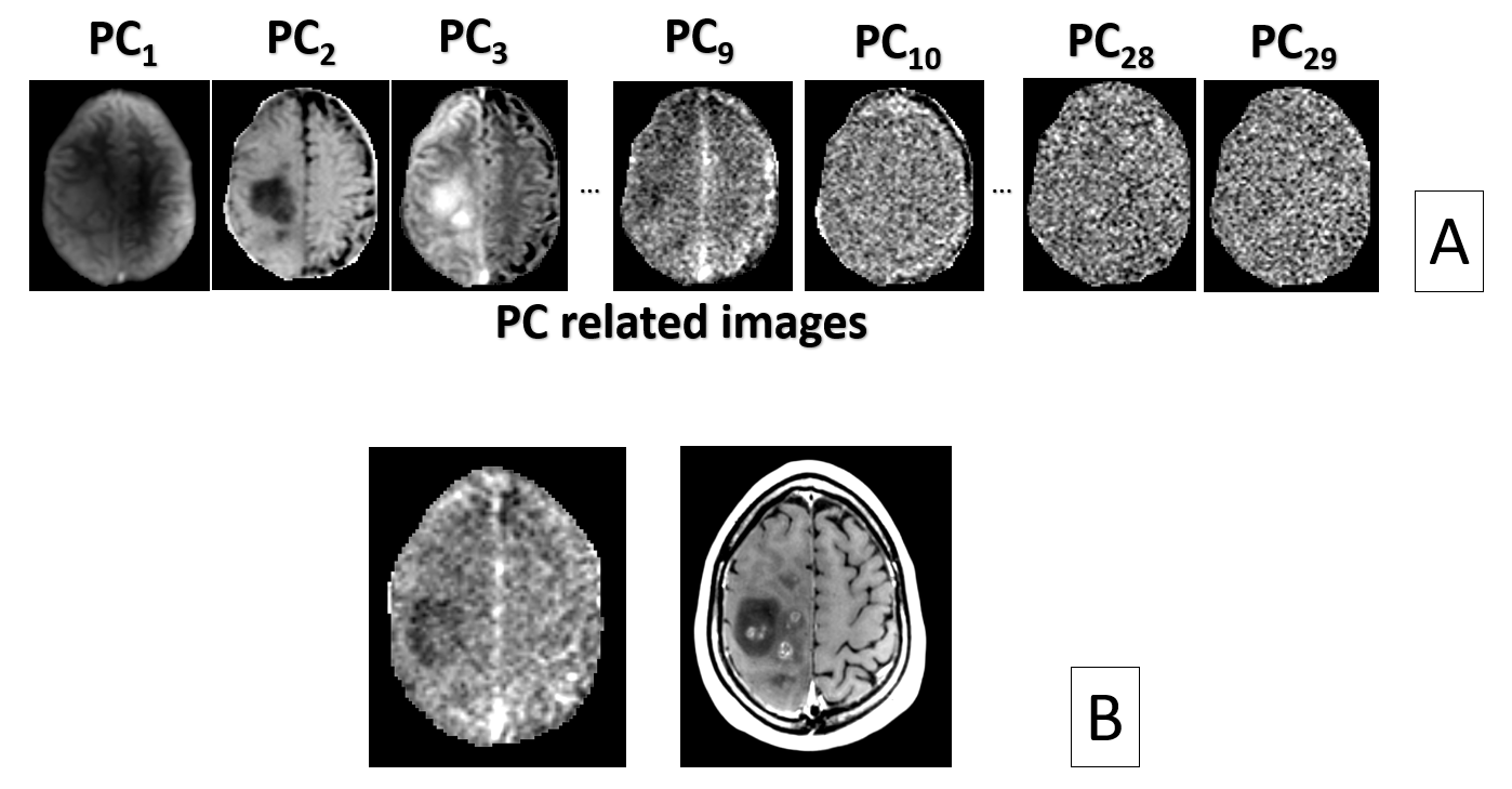
Figure1: A) Example of extracted PC related images of a glioma patient. PC1 until PC3 clearly contain spatial information while PC28 and PC29 contain only noise. PC9 and PC10 however, contain both noise and spatial information. B) PC related image that has been discarded by an eigenvalue-based method (left), although it contains brain tumor related information in agreement with the contrast-enhanced T1-weighted map (right).
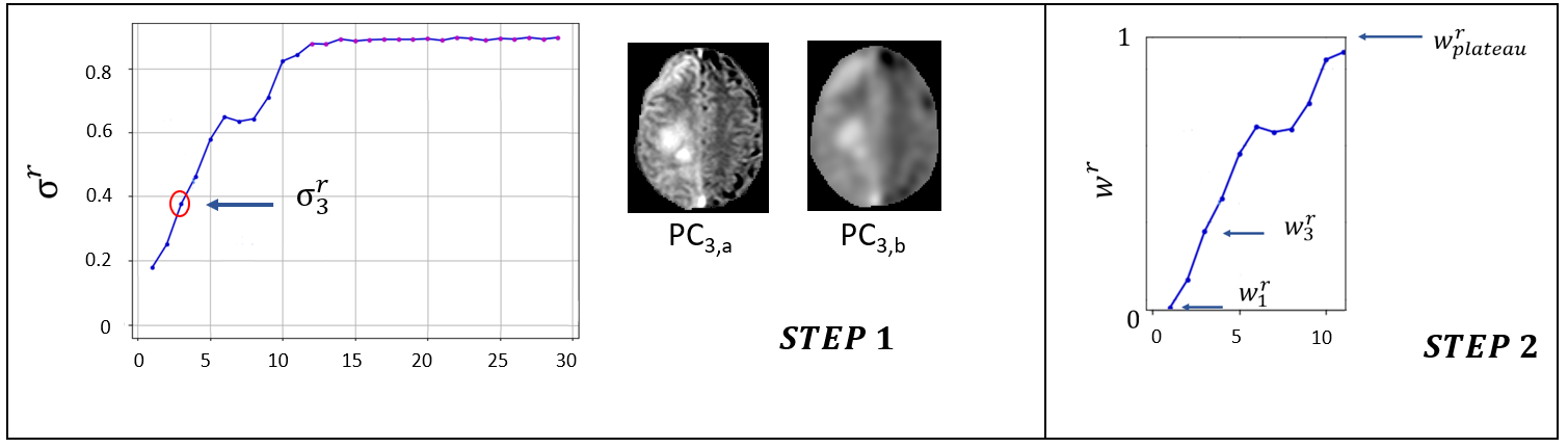
Figure2: Step1: on the PC3 related volume is applied a Gaussian filter and the standard deviation is measured on the image before and after smoothing. In this way $$$\sigma_r3$$$ is calculated. The components with $$$\sigma_r$$$ on the convergence point (purple points on the plateau) are discarded assuming that contain only noise.
Step2: The retained PC related volumes are spatially denoised with a gaussian filter of strength A multiplied by their weights. For example PC3 related volume is smoothed with strength $$$A \cdot w^r_3$$$. $$$A=0.5$$$ was used for this study.
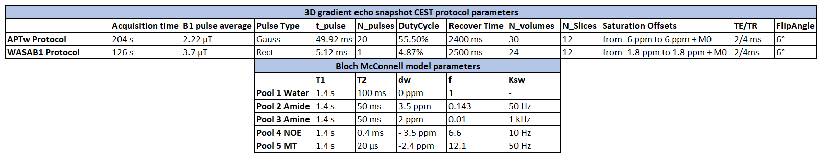

Figure4: Quantitative analysis of the performance of the PCA denoising methods on MTRAsym maps of different SNR levels: A) Peak signal-to-noise ratio (PSNR), B) Structural Similarity Index (SSIM), C) Correlation, D) Mean Square Error (MSE).