2079

Robust Lorentzian fitting of CEST spectra utilizing joint spatial regularization

Oliver Maier¹, Moritz Simon Fabian^2,3, Angelika Barbara Mennecke², Manuel Schmidt², Arnd Dörfler², Kristian Bredies⁴, Moritz Zaiss^2,3, and Rudolf Stollberger^1,5
¹Institute of Medical Engineering, Graz University of Technology, Graz, Austria, ²Department of Neuro-radiology, University Clinic of Erlangen, Erlangen, Germany, ³Friedrich-Alexander-University, Erlangen, Germany, ⁴Institute of Mathematics and Scientific Computing, University of Graz, Graz, Austria, ⁵BioTechMed Graz, Graz, Austria

Synopsis

Chemical Exchange Saturation Transfer (CEST) enables characterization of tissue in vivo by measuring a z-spectrum. Quantitative separation of individual contributions to this spectrum is performed by fitting several Lorentzian shaped lines to the acquired data. Current implementations of the fitting procedure suffer from poor SNR and ambiguity of peaks lying close to each other. To this end, we propose to include a joint spatial regularization to the fitting process to counter the poor SNR and thus improve separation of individual peaks in the final reconstruction.

Indroduction

Chemical Exchange Saturation Transfer (CEST) imaging is based on exchange of mobile water protons between the free water pool and bound water pools on various molecules[1]. In contrast to Magnetic Resonance Spectroscopy Imaging which directly measures the bound protons, CEST utilizes the free water protons to enhance the received signal by several orders of magnitude. The resulting spectrum, the so called z-spectrum, can be described by the Bloch-McConnell equations[2] but solutions to this equations in in vivo settings are infeasible. Thus, a phenomenological description employing several pools of Lorentz shaped functions is typically used to quantify contributions of different molecules[3]. The quantification process can suffer from poor SNR and ambiguity between peaks lying close to each other in the z-spectrum. To improve this process and counter the poor SNR of individual parameters we propose to include a joint spatial regularization term into the fitting process to take advantage of spatial information across all individual maps.

Methods

To identify the contributions of different metabolites to the CEST spectrum a 5-pool Lorentzian model is employed [3]. Each Lorentz function $$$L_i(\omega)$$$ has the following form
$$L_i(\omega)=a_i \frac{(\Gamma_i/2)^2}{(\Gamma_i/2)^2+(\omega-\omega_{0i})^2)}$$
where $$$a_i$$$ describes the scaling, $$$\Gamma_i$$$ the width, $$$\omega$$$ the offset frequency in the z-spectra, and $$$\omega_{0i}$$$ the spectral position of each peak. The five pools are assumed to correspond to water, amide, nuclear Overhauser effect (NOE), magnetization transfer (MT), and amine contributions[4].The parameter of the individual Lorentz functions are identified via a non-linear optimization problem
$$\underset{x}{\min}|| A(x) – d||_2^2 + \lambda TGV_J(x)$$
which is combined with joint total generalized variation ($$$TGV_J$$$) regularization[5,6,7] to utilize spatial information from all estimated parameter maps. $$$A(x)$$$ describes the non-linear forward operator, consisting of the sum of the five Lorentz functions in conjunction with the unknown parameters $$$x=(a_i,\Gamma_i,\omega_{0i})_{i=1,...,5}$$$, $$$d$$$ are the measured z-spectra, and $$$\lambda>0$$$ balances between data and regularization. The proposed regularization strategy has been successfully applied in various quantitative MRI problems[7,8,9], showing increased noise suppression while maintaining small image details.
The resulting problem is solved using an iteratively regularized Gauss-Newton (IRGN) approach combined with a primal-dual splitting algorithm[10,11].Fitting was performed on a GPU using a previously proposed Python toolbox[11], specifically designed to cope with parameter quantification tasks from noisy measurements. The proposed approach was compared to standard pixel-wise fitting of the same five pool Lorentzian model using a Levenberg-Marquardt approach with Matlab (Mathworks).

Data was acquired at a MAGNETOM Terra 7 Tesla scanner (Siemens Healthcare GmbH, Erlangen, Germany) with an 32ch Rx and 8ch head coil. Pre-saturation was realized using the MIMOSA scheme (120 pulses, tp=15 ms, duty cycle DC=60.56%, B1 =0.72µT and 1 µT)[12], followed by a centric 3D snapshot GRE (TE=1770ms, TR=3700ms, FA=6°, FOV=230x186.875x21mm, matrix size104x128x18)[13]. GRAPPA 2 was applied in the first phase encoding direction[14]. Total acquisition time was 13min 24s.
The evaluation of CEST data was done according to [4,15]including motion correction, normalization, denoising, and B1 correction. Linear interpolation between the two B1 stacks using the B1-MIMOSA map corrected for B1 inhomogeneity[12].

Results and Discussion

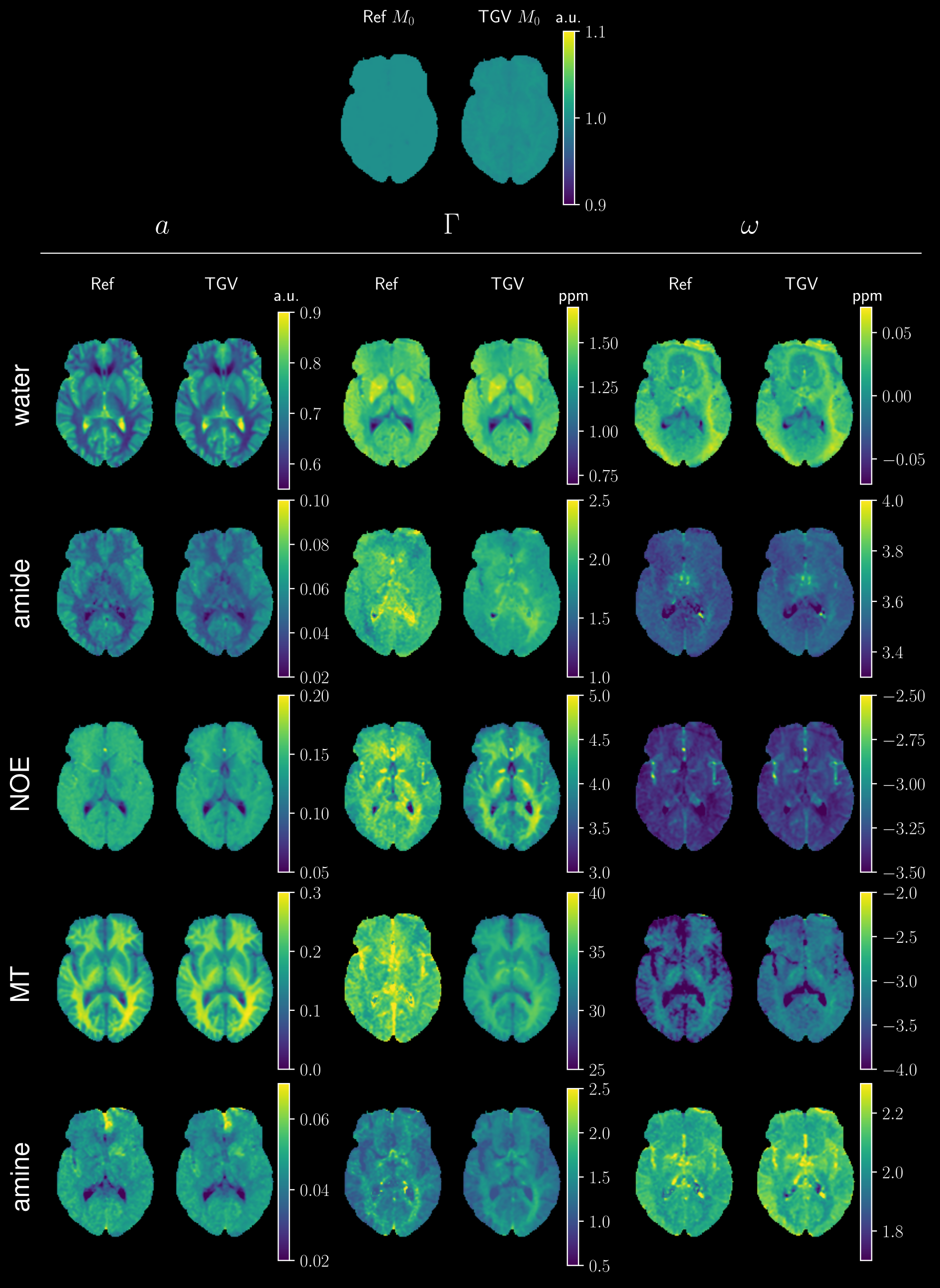
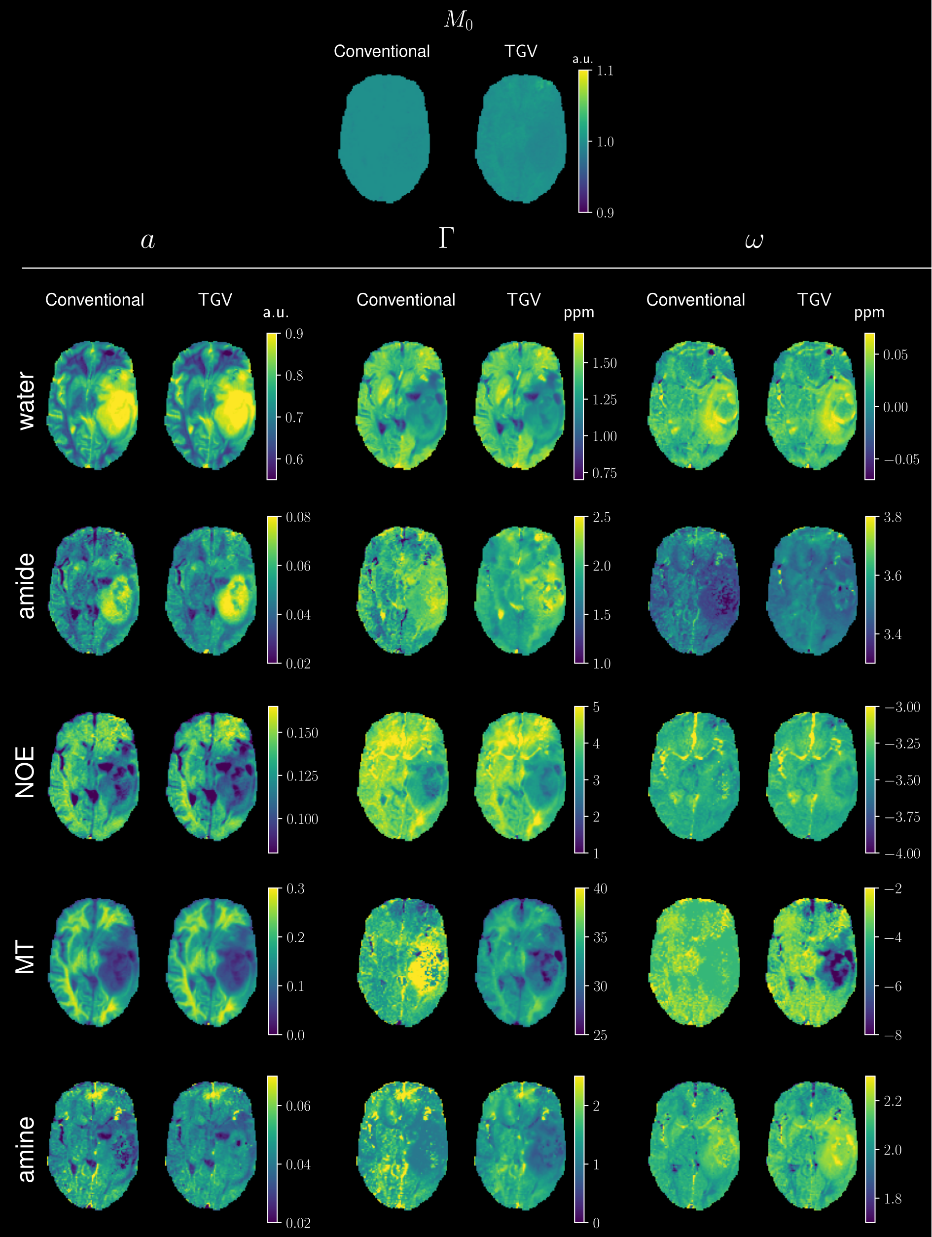
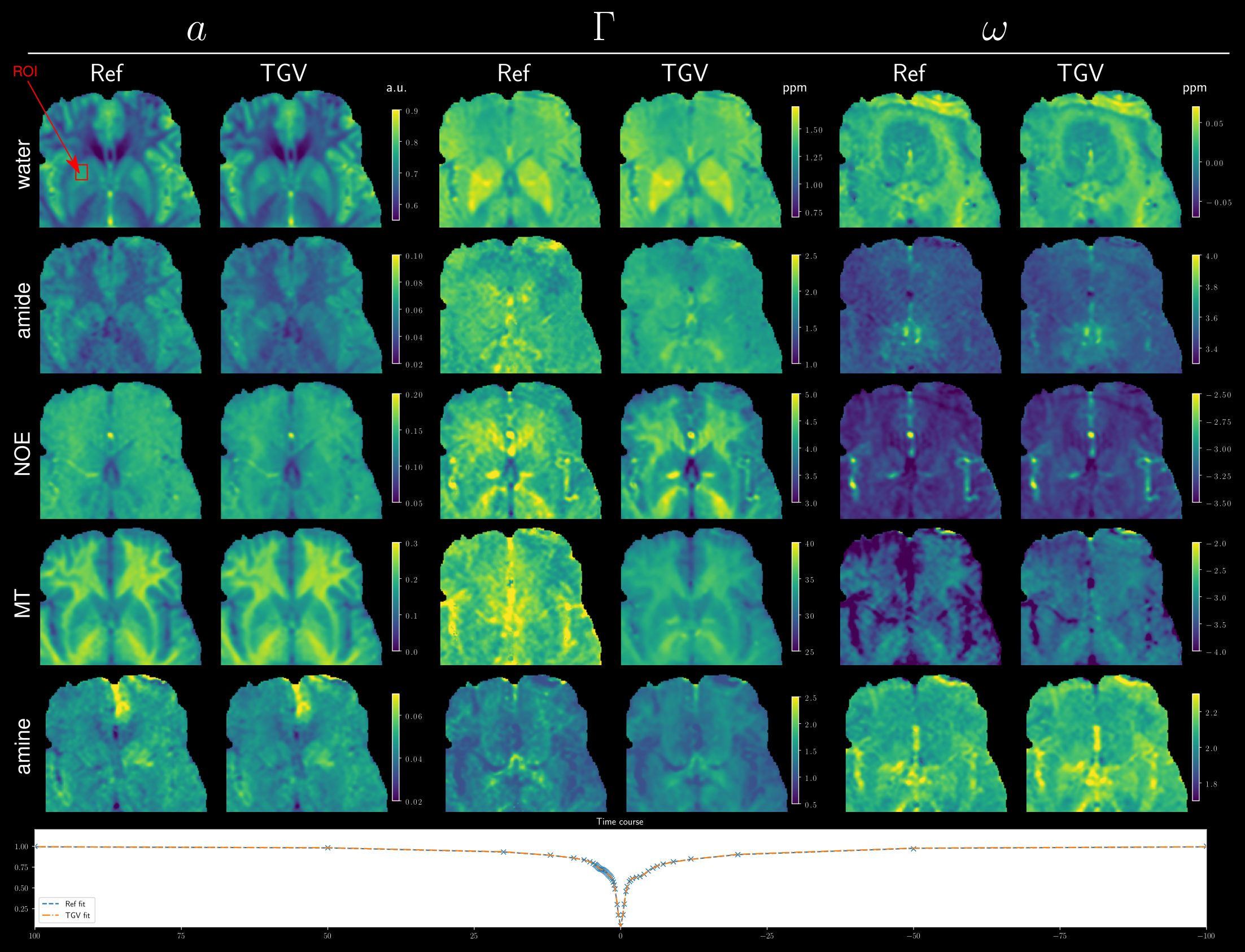
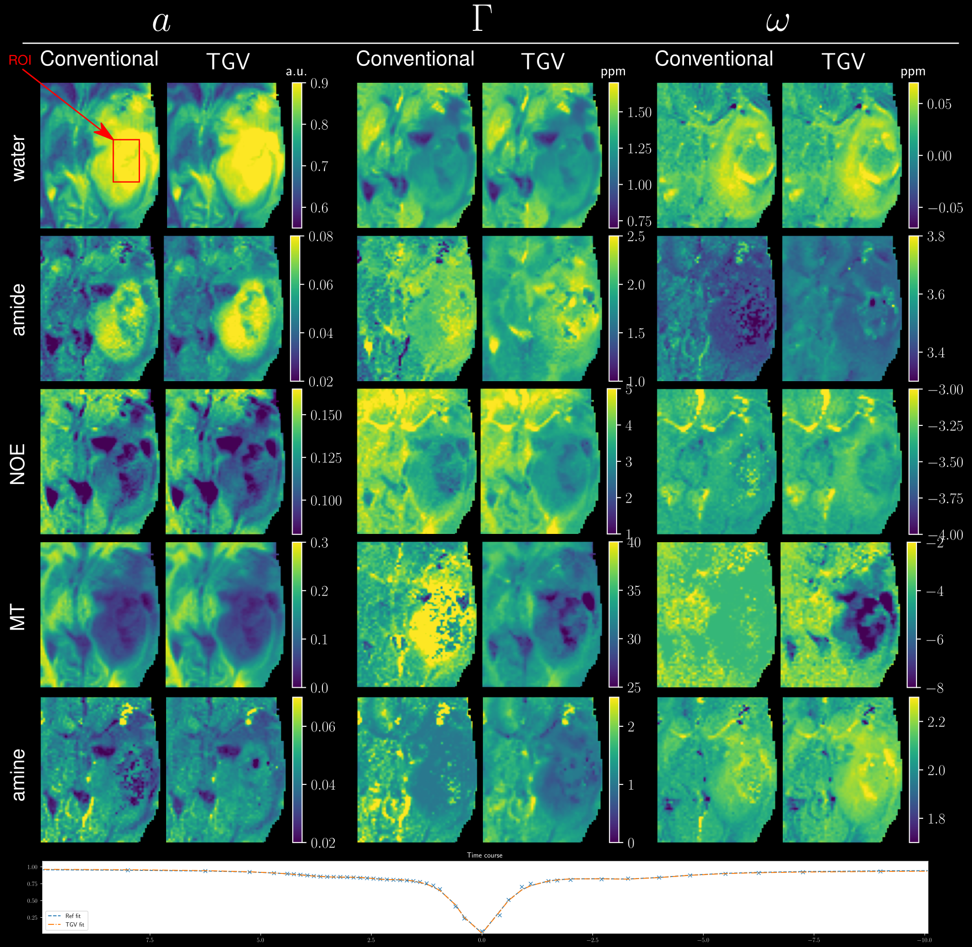
Figure 1 gives an overview of the fitted Lorentz parameters for an exemplary slice of a healthy volunteer. An overview of an exemplary slice for a tumor patient is given in Figure 2. The proposed method exhibits reduced noise while maintaining sharp edges between tissue. Especially noise in the width parameter of each Lorentz pool could be substantially reduced compared to standard pixel-wise fitting. A zoomed view in Figure 3 confirms the de-noising properties of the proposed method, showing reduced noise in nearly all parameter maps. The joint $$$TGV_J$$$ regularization is able to enhance structural information, showing clear boundaries between white and gray matter. Especially tissue boundaries in the width parameter $$$\Gamma$$$ can be detected with the proposed method and are in line with the underlying morphology. Coefficient-of-determination (R²) for the volunteer/patient was 0.997/0.997 and 0.995/0.994 for the conventional and proposed method, respectively. Slightly higher values of the conventional method might indicate over-fitting the data which would be supported by the increased noise in the conventional fitted parameter maps. All tumor features are still visible in the TGV reconstruction, moreover, especially the low intensity amine signal, which is closest to the direct water saturation now shows improved quality outlining the tumor area nicely (Figure 4).

Conclusion

We have shown that the proposed fitting method with joint spatial $$$TGV_J$$$ regularization improves parameter fitting stability for a five pool Lorentzian model reflected by a reduction of noise in the estimated quantitative maps. Further, reconstructed maps maintain high quantitative accuracy and show structures between gray and white matter previously buried in noise. Future work will focus on including the MRI acquisition operator in the fitting process to enable accelerated data acquisition.

Acknowledgements

NVIDIA Corporation Hardware grant support.

References

1. Smith S A, et al. "Pulsed magnetization transfer imaging with body coil transmission at 3 Tesla: Feasibility and application." In: Magn. Reson. Med. (2006), 56: 866-875. doi: 10.1002/mrm.21035

2. McConnell H M "Reaction Rates by Nuclear Magnetic Resonance." In: The Journal of Chemical Physics 28.3 (Mar. 1958), pp. 430-431. doi: 10.1063/1.1744152.

3. Zaiss M, Schmitt B, Bachert P. "Quantitative separation of CEST effect from magnetization transfer and spillover effects by Lorentzian-line-fit analysis of z-spectra." In: J Magn Reson. 2011 Aug;211(2):149-55. doi: 10.1016/j.jmr.2011.05.001.

4. Khakzar K M, et al. "7 tricks for 7T CEST – improving reproducibility of multi-pool evaluation." In: 8th International Workshop on Chemical Exchange Saturation Transfer Imaging, 2020.

5. Bredies K, Kunisch K, and Pock T. "Total generalized variation." In: SIAM Journal on Imaging Sciences 3.3 (Jan. 2010), pp. 492-526. doi: 10.1137/090769521.

6. Huber R, et al. "Total generalized variation regularization for multi-modal electron tomography". In: Nanoscale 11.12 (2019), pp. 5617-5632. doi: 10.1039/c8nr09058k.

7. Maier O, et al. "Rapid T1 quantification from high resolution 3D data with model-based reconstruction". In: Magn. Reson. Med. 81.3 (Oct. 2019), pp. 2072-2089. doi: 10.1002/mrm.27502.

8. Maier O, et al. "Non-linear fitting with joint spatial regularization in arterial spin labeling". In: Med Image Anal 71 (July 2021), p.102067. doi: 10.1016/j.media.2021.102067.

9. Bödenler M, et al. "Joint multi-fieldT1 quantification for fast field-cycling MRI." In: Magn. Reson. Med. (June 2021). doi: 10.1002/mrm.28857.

10. Chambolle A and Pock T. "A first-order primal-dual algorithm for convex problems with applications to imaging." In: Journal of Mathematical Imaging and Vision 40.1 (2011), pp. 120-145. doi: 10.1007/s10851-010-0251-1.

11. Maier O, et al. "PyQMRI: An accelerated Python based Quantitative MRI toolbox". In: Journal of Open Source Software 5.56 (Dec. 2020), p. 2727. doi: 10.21105/joss.02727.

12. Liebert A, et al. "Multiple interleaved mode saturation (MIMOSA) for B1+ inhomogeneity mitigation in chemical exchange saturation transfer". In: Magn Reson Med. 2019 Aug;82(2):693-705. doi: 10.1002/mrm.27762.

13. Zaiss M, Ehses P, and Scheffler K. "Snapshot-CEST: Optimizing spiral-centric-reordered gradient echo acquisition for fast and robust 3D CEST MRI at 9.4 T." In: NMR in Biomedicine 2018;31:e3879 doi: 10.1002/nbm.3879

14. Griswold M A, et al. "Generalized autocalibrating partially parallel acquisitions (GRAPPA)." In: Mag. Reson. Med 47.6 (2002): 1202-1210. doi: 10.1002/mrm.10171

15. Windschuh J, et al. “Correction of B1-inhomogeneities for Relaxation compensated CEST imaging at 7 T”. In: NMR in biomedicine 28.5 (2015), pp. 529–537. doi: 10.1002/nbm.3283

Figures

Figure 1: Parameters of the five pool Lorentzian model for healthy volunteer 1. The scaling parameter $$$a$$$ is given relative to the water signal $$$M_0$$$ which is normalized to one. The conventional fit is given in the left columns and the proposed $$$TGV_J$$$ regularized fit in the right columns for each parameter. A zoomed view is given in Figure 3.

Figure 2: Parameters of the five pool Lorentzian model for a patient suffering from cancer. The scaling parameter $$$a$$$ is given relative to the water signal which is $$$M_0$$$ normalized to one. The conventional fit is given in the left columns and the proposed $$$TGV_J$$$ regularized fit in the right columns for each parameter. Note that the minimum allowed value for $$$\omega$$$ in the MT pool was lowered for the proposed method, thus differences appear larger.

Figure 3: Zoomed view of Figure 1. The proposed method shows reduced noise, especially in the width parameter $$$\Gamma$$$ of the individual Lorentz functions. The bottom part of the figure shows the mean acquired and fitted signal in the marked ROI, given in the top left corner of the figure, for the conventional and proposed method.

Figure 4: Zoomed view of Figure 2. The proposed method shows reduced noise, especially in the width parameter $$$\Gamma$$$ of the individual Lorentz functions and within the amide pool. The bottom part of the figure shows the mean acquired and fitted signal in the marked ROI, given in the top left corner of the figure, for the conventional and proposed method. Note that the spectral range is cut to -10 to 8 ppm to give a more detailed view of the spectrum close to the water peak.

Proc. Intl. Soc. Mag. Reson. Med. 30 (2022)

2079

DOI: https://doi.org/10.58530/2022/2079