2066
Local Integral EPT - the alter ego of Helmholtz EPT1INRIM, Torino, Italy
Synopsis
A local-integral solution of the Electric Properties Tomography (EPT) problem is proposed. The method exploits a trick to consider the Helmholtz equation that regulates EPT as a Poisson equation. Then, it inverts the equation under the local homogeneity assumption, using Green's theorem. The approach turns out to be equivalent to the traditional Helmholtz-EPT.
INTRODUCTION
MR-based Electric Properties Tomography (EPT) is a family of techniques that perform the indirect measurement of the dielectric parameters (conductivity σ and permittivity ε) of the biological tissues, pixel by pixel (or voxel by voxel, in 3D) within the tomographic image, starting from some other measurements carried out through the MRI scanner1. One of the most popular EPT techniques is Helmholtz-EPT2, which relies on the local homogeneity assumption (i.e. it assumes that the gradient of the dielectric parameters is negligible) and then solves the complex Helmholtz equation$$Eq.1\dashrightarrow\triangledown^2B_1^+=-\omega^2\mu(\epsilon-j\sigma/\omega)B_1^+$$
(where μ: magnetic permeability, ω: angular frequency, j: imaginary unit) by direct differentiation of the spatial distribution of the rotating component ($$$B_1^+$$$) of the radiofrequency magnetic flux density, expressed as a complex number.
Here we propose to solve the same equation using another procedure, based on Green's theorem, to investigate the possibility to improve the EPT reconstruction.
METHODS
If the right-hand side of Eq.1 were a known term ζ, it could be seen, formally, as a Poisson equation. By virtue of Green’s second identity, an integral representation for the solution of Eq.1, in a generic point P within a homogeneous region V surrounded by a closed surface S, is3$$Eq.2\dashrightarrow B_1^+(P)=\oint_S \left [B_1^+\frac{\text{d}}{\text{d}n}\left(\frac{1}{4\pi r}\right)-\frac{1}{4\pi r} \frac{\text{d}B_1^+}{\text{d}n}\right]ds+\int_{V}\frac{\zeta}{4\pi r}dv$$
where r is the distance between P and the generic integration point and n indicates the inward direction normal to S.
Since ζ is proportional to $$$B_1^+$$$, Eq.2 can be inverted to get the value of the dielectric parameters in point P:
$$Eq.3\dashrightarrow \epsilon-j\frac{\sigma}{\omega}=\frac{B_1^+(P)-\oint_S\left [B_1^+\frac{\text{d}}{\text{d}n}\left (\frac{1}{4\pi r}\right)-\frac{1}{4\pi r} \frac{\text{d}B_1^+}{\text{d}n}\right]ds}{\omega^2\mu\int_{V} \frac{B_1^+}{4\pi r}dv}$$
As for Helmholtz-EPT, if the magnitude of $$$B_1$$$ is quite uniform around P, an approximated reconstruction of the only conductivity, based on the transceive phase $$$\psi^\pm$$$, is also possible2, starting from the relation $$$\triangledown^2\psi^\pm=2\omega\mu\sigma$$$, which, in the framework of Green’s theorem leads to
$$Eq.4\dashrightarrow \sigma=\frac{\oint_S\left[\psi^\pm\frac{\text{d}}{\text{d}n}\left(\frac{1}{4\pi r}\right)-\frac{1}{4\pi r} \frac{\text{d}\psi^\pm}{\text{d}n}\right]ds-\psi^\pm(P)}{2\omega\mu\int_{V} \frac{1}{4\pi r}dv}$$
The proposed integral solutions hold for any homogeneous region. In particular, they can be applied to each single voxel in the domain, obtaining a local-integral EPT. In this case, the value of the field (or its phase) in point P can coincide with the acquisition performed in a given point of the image (i.e. at the centre of the voxel). The values needed to perform the integrations can be obatined from the samples acquired around such a point, for instance by interpolation (and calculation of the normal derivatives required by Green's identity). The integration can be performed according to different numerical schemes, based on the required level of approximation.
If the Savitzky–Golay filter4 is applied to the field distribution around the computational point (as usually done in Helmholtz-EPT to mitigate the impact of the measurement noise), an approximated analytical description of $$$B_1^+$$$ (or, analogously, of its phase) in a three-dimensional space is obtained in the form of the paraboloid:
$$Eq.5\dashrightarrow B_1^+(x,y,z)=k_1+k_2x+k_3y+k_4z+k_5x^2+k_6y^2+k_7z^2+k_8xy+k_9xz+k_{10}yz$$
that provides the best fitting of the measurements in the least squares sense. Incidentally, this representation allows developing the local-integral EPT in closed form, avoiding any numerical integration.
RESULTS AND DISCUSSION
When the field (or the phase) is represented through the paraboloid indicated in Eq.5, the most natural way to perform the integrations required by Eq.3 (or Eq.4) is in spherical coordinates$$x=r\sin\theta\cos\phi$$ $$y=r\sin\theta\sin\phi$$ $$z=r\cos\theta$$
choosing for volume V a sphere with radius R, centered in point P ($$$\theta$$$: colatitude, $$$\phi$$$: longitude).
The analytical calculation of the three integrals involved in Eq.3, taking into account that $$$\frac{\text{d}}{\text{d}n}\left(\frac{1}{4 \pi r}\right)=-\frac{\text{d}}{\text{d}r}\left(\frac{1}{4 \pi r}\right)=\frac{1}{4 \pi r^2}$$$, is reported in Fig.1, where it becomes clear that some fitting coefficients do not provide any contribution.
Bringing these results into Eq.3, substituting $$$B_1^+(0,0,0)=k_1$$$, and shrinking the sphere around point P (i.e. taking the limit for $$$R\rightarrow0$$$), we get for the dielectric properties the closed form
$$Eq.6\dashrightarrow \epsilon-j\frac{\sigma}{\omega}=-\frac{2}{\omega^2\mu}\frac{k_5+k_6+k_7}{k_1}$$
Equation 6 (where the numerator approximates the Laplacian operator of Eq.1) coincides with the expression used in Helmholtz-EPT combined with the Savitzky-Golay filter, proving the equivalence of the two formulations on the analytical side and legitimating the trick to solve Eq.1 as a Poisson equation.
To compare the two EPT approaches from the numerical viewpoint, synthetic noiseless data have been produced by simulating a human head (resolution: 2 mm) exposed to the field produced by a birdcage coil at 64 MHz. In this case, Eq.3 has been applied to each single voxel in the model, without using any fitting, interpolating the sampled $$$B_1^+$$$ values required for the numerical integrations. Figure 2 shows the maps produced through the two approaches on a slice of the head. An almost perfect consistency (including the typical boundary errors, due to the local homogeneity assumption, of Helmholtz-EPT) is found.
Figure 3 shows the conductivity maps obtained using Eq.4, or Eq.3 applied in 2D (i.e. neglecting the longitudinal derivatives). Both maps agree very well with the analogous Helmholtz-EPT reconstructions.
CONCLUSION
The proposed local-integral version of EPT reveals itself to be a real alter ego of Helmholtz-EPT. The latter suffers from the noise amplification implied by the differentiation process. Hence, future work will investigate whether the natural filtering offered by the spatial integration involved in Eq.3 and Eq.4 can mitigate the noise effectively, without the need for any fitting of the measured data.Acknowledgements
The results here presented have been developed in the framework of the EMPIR Project 18HLT05 QUIERO. This project 18HLT05 QUIERO has received funding from the EMPIR programme co-financed by the Participating States and from the European Union’s Horizon 2020 research and innovation programme.References
1. Leijsen, R.; Brink, W.; van den Berg, C.A.T.; Webb, A.; Remis, R. Electrical properties tomography: A methodological review.Diagnostics 2021;11(2):176.
2. Voigt, T.; Katscher, U.; Doessel, O. Quantitative conductivity and permittivity imaging of the human brain using electric properties tomography. Magn. Reson. Med. 2011;66(2):456–466.
3. Morse, P.M.; Feshbach H. Methods of Theoretical Physics. Mc Graw-Hill Book Company Inc., 1953.
4. Savitzky, A.; Golay, M.J.E. Smoothing and differentiation of data by simplified least squares procedures. Anal. Chem. 1964;36(8):1627–1639.
5. Arduino A. EPTlib: An Open-Source Extensible Collection of Electric Properties Tomography Techniques. Applied Sciences. 2021;11(7):3237.
Figures
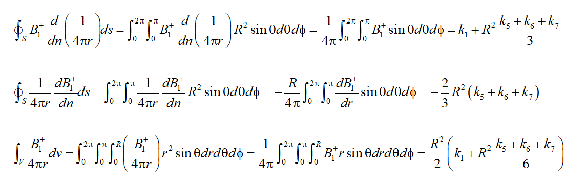


Figure 3 - Conductivity maps obtained through different versions of local-integral EPT.
On the left, the map obtained working with Eq.4 (pahse-based approximation, using the transceive phase as an input).
On the right, the map obtained working with Eq.3 applied in 2D (i.e. neglecting the longitudinal derivatives). The corresponding maps obtained through Helmholtz-EPT (not reported) are almost identical.
With respect to the results in Fig.2, the phase-based version produces a slight over-estimation, whereas the 2D version produces a more blurred map.