1986
A CNN for Oxygen Extraction Fraction Mapping with combined QSM and qBOLD1Computer Assisted Clinical Medicine, Medical Faculty Mannheim, Heidelberg University, Mannheim, Germany
Synopsis
MRI-based mapping of oxygen extraction fraction with QSM and qBOLD is a non-invasive diagnostic tool with many possible applications. But current reconstruction methods based on quasi-Newton (QN) methods are very dependent on accurate parameter initialization. Artificial Neural Networks showed a lot of potential in our previous works. Using a Convolutional Neural Network improves the reconstruction, since neighboring voxels can provide additional information. Using a GESFIDE sequence to sample the qBOLD signal instead of a standard mGRE that samples only the FID, improves the reconstruction accuracy of R2, Y and χnb a lot.
Introduction
The oxygen extraction fraction is an important indicator for the state of tissue in many pathologies, for example cancer1 or stroke2. Various MRI based OEF mapping methods have been developed in recent years, one of them uses a combination of Quantitative Susceptibility Mapping (QSM) and quantitative BOLD (qBOLD)3. An advantage of this method is, that it does not require to subject the patient to a hypercapnic or hyperoxic gas challenge4. But the results of the iterative reconstruction with a quasi-Newton (QN) method strongly depend on the parameter values used for initialization. One recent approach is to replace the QN fit with an artificial neural network (ANN)5. This does not depend on initial values like the fit methods. The reconstruction accuracy strongly depends on the sampling strategy of the qBOLD signal. A GESFIDE6 sequence provides more information about R2 than a standard mGRE sequence that only samples the FID. Replacing the fully connected ANN with voxelwise input by a convolutional neural network (CNN) with image slices as input gives additional noise resistance.Methods
Both the ANN5 and the CNN were trained with artificial data based on the QSM+qBOLD model3.The ANN5 is a MATLAB fitnet, which gets data from each voxel as independent input. For each sample used to train the ANN, transverse relaxation rate R2, venous blood oxygenation Y, volume percentage of voxel filled by deoxygenated blood ν and susceptibility of non blood tissue χnb were drawn from gaussian distributions with approximate mean values R2=15 Hz, Y=60%, ν=3% and χnb =-40 ppb. More details in the ANN paper5. Then the parameters were used to calculate the qBOLD and QSM signal and used as targets for the training. The qBOLD signal was calculated for 8 gradient echoes like in the example shown in Figure 1, normed to 1 at the first gradient echo and gaussian noise was added for an SNR of 100. The ANN was trained with 107 samples.
For the CNN patches of 30*30 pixels were taken from a segmented brain7. Then for each tissue type in the patch a random combination of the five parameters was chosen from uniform distributions in the ranges shown in figure 4. The qBOLD signal was calculated for a GESFIDE sequence with 16 echoes as shown in Figure 1. Gaussian noise was added to qBOLD and QSM data so that SNR=100. Figure 2 shows the CNN architecture, which was realized with Keras and TensorFlow. The CNN was trained with approximately 200,000 patches.
Results
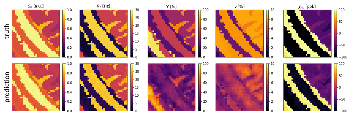
Figure 3 and 4 show 2D histograms of the true parameters used to generate the test data versus the parameter values predicted by the ANN and CNN. This kind of plot gives a much clearer image about a networks performance than a relative error for each parameter. If the reconstruction is perfect it should show a diagonal line through the histogram. For the ANN S0 is very close to the ideal. R2 and χnb are diagonals, but with a very wide spread. Y and ν are not diagonal and show hot spots at the mean values of their training data. The CNN performs much better with very clear diagonal lines for S0, R2 and χnb. Y also shows a lot of improvement with a clear diagonal pattern, but still with a wide spread. v still tends to stick to 3%, although the CNN was trained with v uniformly distributed between 0.1% and 10%.Figure 5 shows parameter maps for an example patch used to test the CNN. Predicted S0, R2 and χnb are very close to the truth with little noise. Y looks blurrier, but shows similar contrast to the truth. ν lacks contrast and detail.
Discussion
GESFIDE leads to much better R2 reconstruction, which in turn makes the reconstruction of Y and χnb much better. ν does not get reconstructed below 2% and for higher true values of v the prediction seems to sometimes be on the diagonal and sometimes stick to 3%. The inverse QSM equation to reconstruct ν from QSM, Y and χnb is a fraction and has a singularity for certain combinations of QSM, Y and χnb. It appears reasonable that the CNN has difficulty to learn the correct function and instead sticks to a mean value for all combinations of QSM, Y and χnb.Conclusion
GESFIDE has significant advantages over mGRE, improving the reconstruction of all parameters except ν. For OEF mapping we are especially interested in the venous oxygen saturation Y, since OEF=(Ya-Yv)/Ya . So this big improvement in Y from the ANN to the CNN is very promising. Currently we are preparing to measure test subjects with such a sequence to compare the CNN results to previous works and other methods.Acknowledgements
No acknowledgement found.References
1. Vaupel P, Mayer A. Hypoxia in cancer: significance and impact on clinical outcome. Cancer Metastasis Rev 2007;26(2):225-239.
2. Ibaraki M, Shimosegawa E, Miura S, Takahashi K, Ito H, Kanno I, Hatazawa J. PET measurements of CBF, OEF, and CMRO2 without arterial sampling in hyperacute ischemic stroke: method and error analysis. Ann Nucl Med 2004;18(1):35-44.
3. , , , , , . Comparison of gradient echo and gradient echo sampling of spin echo sequence for the quantification of the oxygen extraction fraction from a combined quantitative susceptibility mapping and quantitative BOLD (QSM+qBOLD) approach. Magn Reson Med 2019;82:1491-1503.
Cho, J, Ma, Y, Spincemaille, P, Pike, GB, Wang, Y. Cerebral oxygen extraction fraction: Comparison of dual‐gas challenge calibrated BOLD with CBF and challenge‐free gradient echo QSM+qBOLD. Magn Reson Med. 2020; 85: 953– 961.
5. , , , , , . Using an artificial neural network for fast mapping of the oxygen extraction fraction with combined QSM and quantitative BOLD. Magn Reson Med. 2019; 82: 2199– 2211.
6. Ma, J, Wehrli, F. Method for Image-Based Measurement of the Reversible and Irreversible Contribution to the Transverse-Relaxation Rate. J. Magn. Reson. B 1996; 111:61
7. . Med Image Anal.
Figures
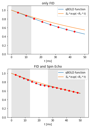
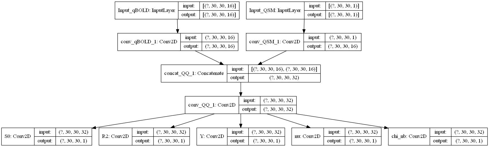
Fig. 2: Architecture of the CNN: A patch of 30*30 pixels with 16 echoes is used as qBOLD input and a patch of 30*30 pixels as QSM input. Each followed by a convolutional layer with 16 filters, kernel size 3, activation tanh. Then a concatenation to combine QSM and qBOLD and another convolutional layer, this one with 32 filters, kernel size 3 and activation tanh. Finally, 5 output layers with only 1 filter and a linear activation function. The network is fully convolutional and can adjust to different image sizes.
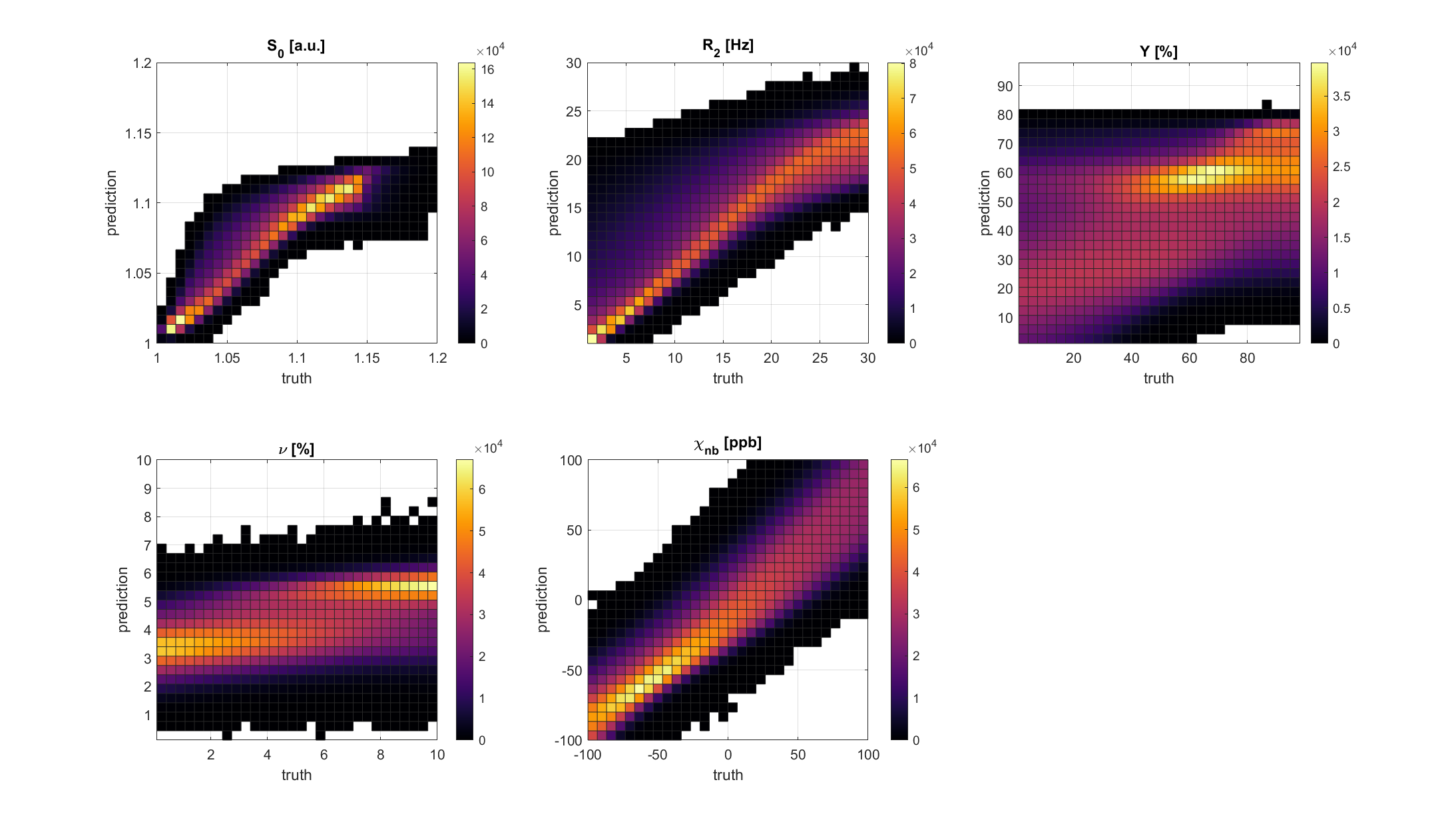
Fig. 3: Results of the ANN5. 2D histograms of the true parameters used to generate artificial data versus the parameter values predicted by the ANN. Input were 10e7 samples of artificial data calculated with random values for R2, Y, ν and χnb, each uniformly distributed in the range shown on the x axis. S0 was adjusted so that the amplitude at the first echo at 4.5 ms is equal to 1. Perfect reconstruction with truth = prediction should be a diagonal line in the histogram. R2 and χnb show diagonals, but not very sharp. Y and ν tend to stick to the mean of their training data at Y=60% and ν=3%.
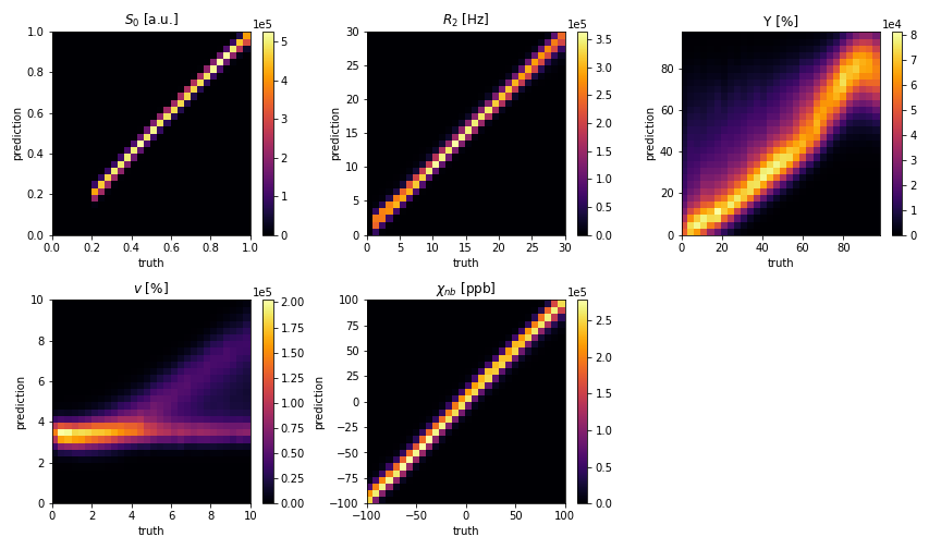
Fig. 4: Results of the CNN. 2D histograms of the true parameters used to generate artificial data versus the parameter values predicted by the ANN. Input were approx. 20,000 patches of artificial data calculated with random values of S0, R2, Y, ν and χnb for each tissue type. On average the parameters were uniformly distributed in the ranges shown on the x axes, except for S0 which was between 0.2 and 1.
GESFIDE sequence leads to much better reconstruction of R2. Also large improvements in χnb. Y is almost a diagonal line, but still spread out. ν tends to be reconstructed between 3 and 4 %.