1983
Development of a Quantitative Susceptibility Mapping (QSM) phantom for validation of acquisition strategies and post-processing tools at 3 T1Centre for Advanced Imaging, The University of Queensland, Brisbane, Australia, 2ARC Training Centre for Innovation in Biomedical Imaging Technology, Brisbane, Australia, 3Siemens Healthcare Pty Ltd, Brisbane, Australia, 4High Field MR Center, Department of Biomedical Imaging and Image-Guided Therapy, Medical University of Vienna, Vienna, Austria, 5Karl Landsteiner Institute for Clinical Molecular MR in Musculoskeletal Imaging, Vienna, Austria, 6Department of Neurology, Medical University of Graz, Graz, Austria, 7School of Information Technology and Electrical Engineering, The University of Queensland, Brisbane, Australia
Synopsis
The phantom was developed to cover the full range of physiological and pathological magnetic susceptibility seen in iron- and calcium-containing tissue, using 4 materials within the one phantom. The phantom facilitates quality assurance for acquisition strategies and post-processing tools.
INTRODUCTION
QSM provides improved detection and differentiation of iron and calcium deposits compared to susceptibility weighted imaging (1), which is important for the diagnosis of neurodegenerative diseases such as Alzheimer’s (2), intracranial haemorrhage staging (3) and brain tumours (4). Due to its complexity, the clinical and MR research communities are actively investigating validation approaches for QSM to verify how the data is acquired, and the uncertainty in how images are post-processed. There are a number of QSM phantoms proposed to date (5–7), yet no one phantom covers the full range of physiological and pathological magnetic susceptibility seen in iron- and calcium-containing tissue (8,9). The project aims to design and prototype such a phantom, facilitating quality assurance for acquisition strategies and post-processing tools for QSM.METHODS
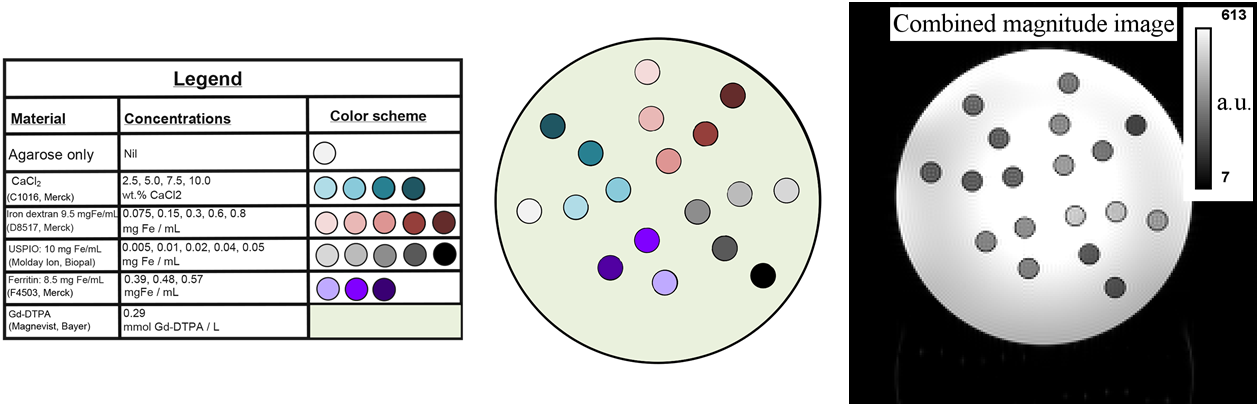
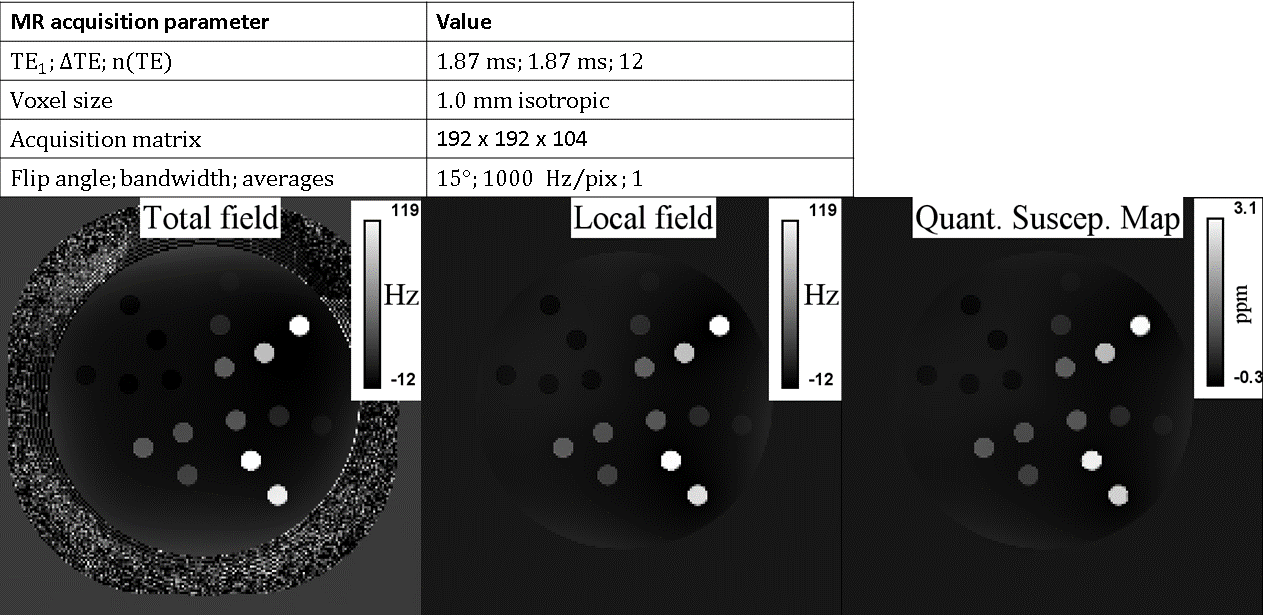
Phantom construction: The phantom (cylinder with outer dimensions: 140 mm diameter, 220 mm length, see cross-section in figure 1) was filled with deionized water and Magnevist (0.29 mmol/L). 18 vials (10 mm diameter) were added, filled with a gel (1.5 wt.% low-melting-point agarose heated to 60°C), and one of the 4 materials with varied concentrations (figure 1). The concentrations were chosen to cover a wide physiological and pathological range of iron- and calcium-containing tissue (8,9). The gel was microwaved in a conical flask and inspected under light to detect clumps within the gel to ensure that the iron and/or calcium had not agglomerated. Bubbles were removed by swirling within the conical flask and over-filling the NMR tube, prior to sealing with the cap. The imaging volume and the fill port volume were separated by an acrylic disk, preventing potential air bubble diffusion into the imaging space. Each vial was positioned ≥ 9 mm away from each other, and ≥ 9 mm away from the phantom periphery.MRI data acquisition: magnitude and phase data were acquired using a bipolar multi-echo GRE acquisition (figure 2) on a 3 Tesla scanner (Magnetom Prisma, Siemens Healthcare, Erlangen, Germany).
QSM reconstruction: coil combination and unwrapping: ASPIRE (10), ROMEO (11); multi-echo combination: unweighted fitting of the unwrapped phase; background field removal: LBV (12); dipole inversion: MEDI (13). The first echo was set as the template for temporal unwrapping (11), and eddy current phase offsets were corrected (10).
Image analysis: Cylindrical ROIs (7 mm) were defined on the magnitude image for each vial in ImageJ over 30 slices about the isocentre, excluding Gibbs’ ringing, partial volume effects at vial boundaries and aliasing artefacts at distal slices. The phase offset ($$$ψ_0$$$) was measured by fitting the unwrapped phase against echo time ($$$ψ = ψ(TE) + ψ_0$$$). R2* map: fast numerical method NumART2* from the magnitude data (14).
RESULTS & DISCUSSION
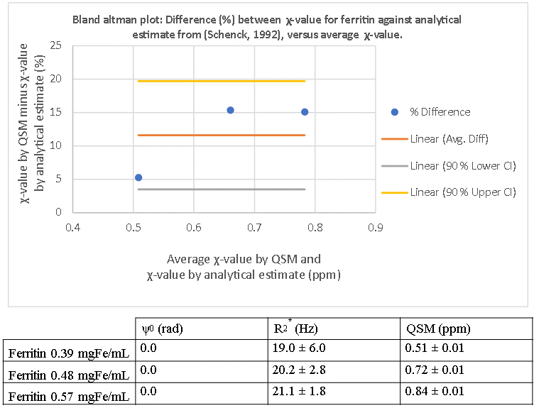
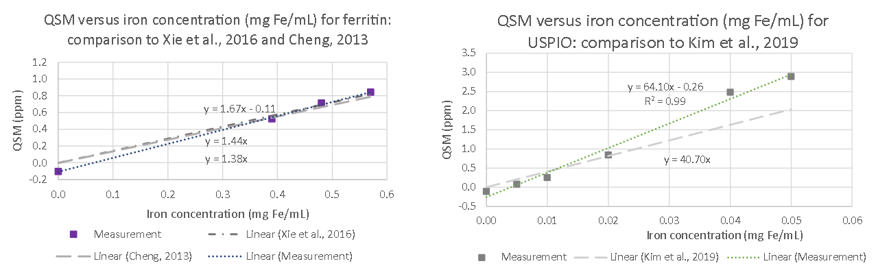
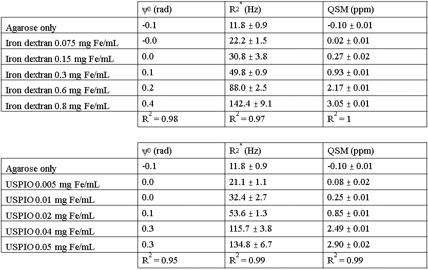
There is visible contrast in the total field, local field and QSM for all iron-based materials, as can be seen in Figure 2. The total field, and to a lesser extent the local field and QSM show inhomogeneities about the phantom periphery. The local field and QSM contrast appear similar.There are a range of factors that might influence a χ-value estimate by QSM. Figure 3 shows that our χ-value estimate by QSM were overestimated by between 5 to 15 % when compared to the analytical χ-value estimate (15); which might be attributed to incomplete background field removal. External reference measurements (e.g., using SQUIDs) could provide further validation. Figure 4 (left and right) shows that our χ-value estimate by QSM is higher compared to other χ-value estimates by QSM (5–7); which might be attributed to differences in acquisition strategies and post-processing parameters. The χ-value estimates for calcium chloride were a factor of 4 lower than literature (7): -0.009 ppm / wt.% CaCl2, likely due to the use of a different solute (granular calcium chloride) as a basis for the gel mixture.
In general, QSM phantom studies need to consider spatial dependencies. Phase offsets might be larger about higher iron concentrations, shown in figure 5. Future phantom designs should integrate multiple samples of the same concentration at different locations.
CONCLUSION
This phantom shows promise to be able to critically assess and verify QSM acquisition strategies and post-processing tools. The phantom can be improved by utilizing more vials of the same concentration distributed across the phantom to reduce potential bias from spatial dependencies.Acknowledgements
We thank the CAI workshop staff for designing and machining the phantom.References
1. Soman S, Lee K, Selim M, Filippidis A, Thomas A, Spincemaille P, et al. Improved Cerebral Microbleed vs Calcification Discrimination using QSM compared to SWI Phase Maps. In: Proceedings of International Society of Magnetic Resonance in Medicine. Virtual Conference; 2020.
2. Ravanfar P, Loi SM, Syeda WT, Van Rheenen TE, Bush AI, Desmond P, et al. Systematic Review: Quantitative Susceptibility Mapping (QSM) of Brain Iron Profile in Neurodegenerative Diseases. Front Neurosci. 2021 Feb 18;15:618435.
3. Chang S, Zhang J, Liu T, Tsiouris AJ, Shou J, Nguyen T, et al. Quantitative Susceptibility Mapping of Intracerebral Hemorrhages at Various Stages. J Magn Reson Imaging. 2016 Aug;44(2):420–5.
4. Deistung A, Schweser F, Wiestler B, Abello M, Roethke M, Sahm F, et al. Quantitative Susceptibility Mapping Differentiates between Blood Depositions and Calcifications in Patients with Glioblastoma. Kleinschnitz C, editor. PLoS ONE. 2013 Mar 21;8(3):e57924.
5. Kim J-H, Kim J-H, Lee S-H, Park J, Lee S-K. Fabrication of a spherical inclusion phantom for validation of magnetic resonance-based magnetic susceptibility imaging. Deniz CM, editor. PLOS ONE. 2019 Aug 5;14(8):e0220639.
6. Xie H, Cheng Y-CN, Kokeny P, Liu S, Hsieh C-Y, Haacke EM, et al. A quantitative study of susceptibility and additional frequency shift of three common materials in MRI: A Quantitative Study of Susceptibility and Additional Frequency Shift. Magn Reson Med. 2016 Oct;76(4):1263–9.
7. Cheng Y-CN. Development and Testing of Iron Based Phantoms as Standards for the Diagnosis of Microbleeds and Oxygen Saturation with Applications in Dementia, Stroke, and Traumatic Brain Injury: [Internet]. Detroit, Michigan: Defense Technical Information Center; 2013 Oct [cited 2021 Nov 1]. Report No.: ADA601806. Available from: https://apps.dtic.mil/sti/citations/ADA601806
8. Oshima S, Fushimi Y, Okada T, Takakura K, Liu C, Yokota Y, et al. Brain MRI with Quantitative Susceptibility Mapping: Relationship to CT Attenuation Values. Radiology. 2020 Mar;294(3):600–9.
9. Sun H, Klahr AC, Kate M, Gioia LC, Emery DJ, Butcher KS, et al. Quantitative Susceptibility Mapping for Following Intracranial Hemorrhage. Radiology. 2018 Sep;288(3):830–9.
10. Eckstein K, Dymerska B, Bachrata B, Bogner W, Poljanc K, Trattnig S, et al. Computationally Efficient Combination of Multi-channel Phase Data From Multi-echo Acquisitions (ASPIRE). Magn Reson Med. 2018 Jun;79(6):2996–3006.
11. Dymerska B, Eckstein K, Bachrata B, Siow B, Trattnig S, Shmueli K, et al. Phase unwrapping with a rapid opensource minimum spanning tree algorithm (ROMEO). Magn Reson Med. 2021 Apr;85(4):2294–308.
12. Zhou D, Liu T, Spincemaille P, Wang Y. Background field removal by solving the Laplacian boundary value problem. NMR Biomed. 2014 Mar;27(3):312–9.
13. Liu J, Liu T, de Rochefort L, Ledoux J, Khalidov I, Chen W, et al. Morphology enabled dipole inversion for quantitative susceptibility mapping using structural consistency between the magnitude image and the susceptibility map. NeuroImage. 2012 Feb;59(3):2560–8.
14. Hagberg GE, Bianciardi M, Patria F, Indovina I. Quantitative NumART2* mapping in functional MRI studies at 1.5 T. Magn Reson Imaging. 2003 Dec;21(10):1241–9.
15. Schenck JF. Health and Physiological Effects of Human Exposure to Whole-Body Four-Tesla Magnetic Fields during MRI. Ann N Y Acad Sci. 1992 Mar;649(1 Biological Ef):285–301.
Figures