Introduction

An outstanding challenge when using Deep Learning (DL) for Diffusion Tensor Imaging (DTI) is the large variability of acquisition settings (e.g. number of q-space samples, gradient directions and strength) between datasets. Existing works^1-3 applied DL to estimate diffusion properties (e.g fractional anisotropy (FA), mean diffusivity (MD)) from diffusion-weighted (DW) images, but different acquisition schemes required training new models.

In this study, we propose to use the Recurrent Inference Machine (RIM) framework⁴ to estimate the diffusion tensor parameters with low dependency on scan settings. RIMs learn to minimize a model-based likelihood function, allowing for greater variability of fixed model parameters (e.g. gradient directions). We evaluated our model in simulation and in-vivo experiments.

Methods

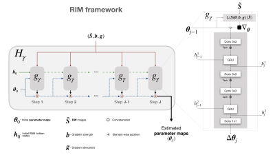
Our RIM for DTI ($$$\textit{dti}\textbf{RIM}$$$) is shown in Figure 1. The RIM is a recurrent neural network $$$\hat{\boldsymbol{\theta}}=H_{\boldsymbol{\gamma}}(\tilde{\boldsymbol{S}};\boldsymbol{b},\boldsymbol{g})$$$ that estimates the diffusion tensor parameters $$$\boldsymbol{\theta}=[S_0,D_{11},D_{12},D_{22},D_{13},D_{23},D_{33}]$$$ using the Rice likelihood $$$L(\boldsymbol{S}(\boldsymbol{\theta};\boldsymbol{b},\boldsymbol{g})|\tilde{\boldsymbol{S}})$$$ w.r.t. the acquired DW images $$$\tilde{\boldsymbol{S}}$$$, where $$$\boldsymbol{b}$$$ is the gradient strength and $$$\boldsymbol{g}$$$ the direction. The network weights $$$\boldsymbol{\gamma}$$$ are trained on simulation data, by minimizing the differences between ground-truth noiseless DW images $$$\boldsymbol{S}^{GT}$$$ and predicted images $$$\boldsymbol{S}(\hat{\boldsymbol{\theta}};\boldsymbol{b},\boldsymbol{g})$$$: $$$\textstyle{\hat{\boldsymbol{\gamma}}=\arg\min_{\boldsymbol{\gamma}}\frac{1}{N}\sum\nolimits_{n=0}^{N-1}(\boldsymbol{S}^{GT}_{n}-\boldsymbol{S}_n(\hat{\boldsymbol{\theta}};\boldsymbol{b},\boldsymbol{g}))^{2}}$$$, where $$$N$$$ is the number of images in the training set.

Training samples $$$T^F_i=\{\tilde{\boldsymbol{S}},\boldsymbol{S}^{GT},\boldsymbol{b},\boldsymbol{g}\}$$$ were generated with the Numerical Fiber Generator⁵ (NFG). For each sample $$$i$$$, $$$\boldsymbol{S}^{GT}$$$ was simulated with uniformly sampled FA$$$\sim\mathcal{U}(0.05,1)$$$ and MD$$$\sim\mathcal{U}(0.0003,0.003)$$$, $$$b=1000s/mm^2$$$, and $$$\boldsymbol{g}$$$ and $$$N$$$ randomly sampled from a pre-determined set $$$\boldsymbol{G}$$$. To ensure approximately uniform sets of gradient directions of size $$$N\in\{7,13,...,55,61\}$$$ (in steps of 6), we selected 10 unique subsets $$$\boldsymbol{g}\in\boldsymbol{G}$$$ with the lowest electrostatic repulsion⁶ among 1000 random subsets of size $$$N$$$. Finally, Rician noise was added. In total, $$$400.000$$$ noisy training samples were created.

Two validation sets were used to tune the RIM's hyperparameters. The first ($$$\textbf{NFG}_{val}$$$) was also created with NFG, but with a different configuration of fibers, $$$\boldsymbol{g}\in\boldsymbol{G},N=31$$$ and SNR 25. The second ($$$\textbf{Diffantom}$$$), was created using the Diffantom simulator⁷, with gradients $$$\boldsymbol{G},N=129,b=2000 s/mm^2$$$ and SNR 30.

In contrast to voxel-wise methods, RIMs also learn a spatial regularization⁸, which might provide robustness to small deviations between signals and the diffusion model. To evaluate this, we created additional $$$\textbf{NFG}_{val}$$$ and $$$\textbf{Diffantom}$$$ datasets with (slightly) misaligned images. Random rigid transformations were applied when generating $$$\tilde{\boldsymbol{S}}$$$ from $$$\boldsymbol{S}^{GT}$$$, with translations and rotations independently sampled from $$$\mathcal{N}(0.0,\sigma_d)$$$, with small $$$\sigma_d=[0.25,0.5]$$$ to simulate sub-voxel misalignment. Fifty realizations of motion and noise were created per dataset. Bias, standard deviation and RMSE of the FA and MD maps were evaluated. Ground-truth maps were defined as the least-squares solution of $$$\boldsymbol{\theta}$$$ on $$$\boldsymbol{S}^{GT}$$$.

The testing data ($$$\textbf{AOMIC}$$$) is composed of 1 subject from the AOMIC-ID1000 dataset⁹, acquired with gradient directions $$$\boldsymbol{G_t}\notin\boldsymbol{G}, N=33, b = 1000 s/mm^2$$$. To evaluate our method's precision, we emulated repeated scans by creating 4 datasets from the original data with varying number of images ($$$N=\{13,19,25,31\},\boldsymbol{g_t}\in\boldsymbol{G_t}$$$). Each contained 5 unique DW sets, with $$$\boldsymbol{g_t}$$$ selected by minimizing the electrostatic repulsion among 100 random subsets of $$$\boldsymbol{G_t}$$$. Ground-truth maps were obtained from the full set ($$$\boldsymbol{G_t}, N=33$$$) with the state-of-the-art $$$\textbf{IWLLS}$$$¹⁰ from MRTrix3¹¹, also used here as baseline in all experiments. Statistical significance was evaluated with an unpaired t-test ($$$p<0.001$$$).

Results

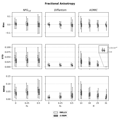
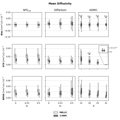
Figure 2 shows the results of FA for all datasets. On $$$\textbf{NFG}_{val}$$$ datasets, $$$\textit{dti}\textbf{RIM}$$$ presented lower bias, STD and RMSE than $$$\textbf{IWLLS}$$$. On $$$\textbf{Diffantom}$$$ datasets, $$$\textit{dti}\textbf{RIM}$$$ had lower STD and RMSE, but higher bias. Additionally, $$$\textit{dti}\textbf{RIM}$$$ errors increased slower than $$$\textbf{IWLLS}$$$ for larger $$$\sigma_d$$$. For $$$\textbf{AOMIC}$$$, $$$\textit{dti}\textbf{RIM}$$$ had lower STD ($$$\forall N$$$), but larger bias and RMSE for $$$N\leq18$$$.

Figure 3 shows the results of MD for all datasets. $$$\textit{dti}\textbf{RIM}$$$ had lower bias, STD and RMSE than $$$\textbf{IWLLS}$$$ in all validation datasets. In $$$\textbf{AOMIC}$$$, $$$\textit{dti}\textbf{RIM}$$$ had lower STD, but higher RMSE compared to $$$\textbf{IWLLS}$$$, while no significant differences were found for bias.

Figures 4 and 5 show FA and MD maps from $$$\textbf{IWLLS}$$$ and $$$\textit{dti}\textbf{RIM}$$$ (data $$$\boldsymbol{G_t}, N=33$$$) alongside RMSE maps computed for different $$$N$$$. $$$\textit{dti}\textbf{RIM}$$$ FA estimates are less dependent on $$$N$$$ than $$$\textbf{IWLLS}$$$'s, while MD maps are smoother, and with lower accuracy in high diffusivity regions (e.g. ventricles).

Discussion

We showed that a single RIM model can be used with DW images acquired with different number of q-space samples, gradient directions and strength. The $$$\textit{dti}\textbf{RIM}$$$ reduced FA and MD errors compared to the state-of-the-art $$$\textbf{IWLLS}$$$ for most datasets. The negative FA bias on in-vivo data can be (mainly) attributed to lower FA estimates in gray matter and CSF, while smaller differences were observed on white matter. MD maps from $$$\textit{dti}\textbf{RIM}$$$ are slightly blurred compared to $$$\textbf{IWLLS}$$$'s, promoting higher estimation precision, at the cost of higher total error. Additionally, (slight) robustness to misaligned images was shown.

Conclusion

This work presented a novel approach to estimate DTI parameters. Our Recurrent Inference Machine method provides estimates with similar or lower error that IWLLS. It showed robustness to anatomy and variation in scan protocol, including q-space sampling.. Although more validation is needed (e.g. larger in-vivo datasets, pathology), our study suggests that the RIM can provide diffusion parameters that are robust and of higher quality than the current state-of-the-art.

Acknowledgements

This project was funded by the European Union’s Horizon 2020 programme, under the grant agreement No 764513.