1909
Analyzing Task-based fMRI Time Series using Machine Learning
Elaine Yuen Fong Kuan1,2, Viktor Vegh1,2, Kieran O'Brien3, Amanda Hammond3, Javier Urriola Yaksic1, and David Reutens1,2
1Centre of Advanced Imaging, The University of Queensland, Brisbane, Australia, 2ARC Training Centre for Innovation in Biomedical Imaging Technology, The University of Queensland, Brisbane, Australia, 3Siemens Healthcare Pty Ltd, Brisbane, Australia
1Centre of Advanced Imaging, The University of Queensland, Brisbane, Australia, 2ARC Training Centre for Innovation in Biomedical Imaging Technology, The University of Queensland, Brisbane, Australia, 3Siemens Healthcare Pty Ltd, Brisbane, Australia
Synopsis
Common approaches for analyzing task-based fMRI data rely upon the use of regressors, which in some experimental paradigms are difficult to define. A machine learning method is proposed to overcome this challenge. Three machine learning methods with established utility for time series classification were used to classify areas of activation and non-activation in a language fMRI study. Machine learning methods were able to identify the activation regions identified by analyses using the General Linear Model (GLM). Machine learning may be useful for fMRI time series analysis, particularly when regressors required for GLM-based analyses are difficult to define.
Introduction
GLM-based analysis of task-based fMRI requires timing information of tasks and parameters from preprocessing to construct regressors1. However, in some experimental paradigms, the regressors are not available or well understood. Analysis also requires data pre-processing and familiarity with dedicated analysis software, which pose challenges for the wide clinical application of fMRI. With recent advances in artificial intelligence, machine learning has become a potentially valuable tool to overcome these challenges2,3. This study explores the feasibility of applying machine learning methods to produce fMRI activation maps for pre-processed time series imaging data, without the use of regressors.Methods
A previously developed block design language fMRI protocol was used4. In 4 participants, 3T gradient echo EPI fMRI data were obtained using the following parameters: matrix size = 64 x 64 x 42, TR = 2s, TE = 30ms and voxel size = 3 x 3 x 3mm3.The raw EPI data were preprocessed (slice timing correction, realignment of volumes, co-registration and smoothing) using Statistical Parametric Mapping (SPM12) software5. Voxel-wise fMRI time series data were modeled with the General Linear Model (GLM) using task and nuisance regressors in SPM12 and voxel activation identified at p < 0.001 uncorrected and p < 0.05 Family Wise Error (FWE) corrected (Figure 1). The thresholded activation maps were then extracted as binary [1,0] maps, with areas of activation labeled as 1 (Figure 2).
At each activation threshold, for 3 participants, time series voxel intensity values from the preprocessed fMRI data were extracted to form the machine learning training set (labeled either 0 or 1 depending on activation; Figure 3). Data from the fourth participant formed the test set. The training and test sets had 673,585 and 207,250 samples respectively. In the training set, 9630 voxels were labeled as 1 and 663,955 were labeled as 0 for SPM12 activation map thresholded at p < 0.001 uncorrected. Using the p < 0.05 FWE corrected threshold, 3230 voxels were labeled as 1 and 670,355 voxels as 0 in the training set. In the test set, 6,266 voxels were labeled as 1 and 200,984 voxels as 0 for SPM12 activation map thresholded at p < 0.001 uncorrected. Using the p < 0.05 FWE corrected threshold, 3,189 voxels were labeled as 1 and 204,061 voxels as 0 in the test set.
Machine learning models were used to classify each voxel based on its fMRI time series to produce activation maps. We evaluated 3 machine learning models with established robustness and utility in time series classification - Random Forest (RF)2,6, Random Interval Spectral Ensemble (RISE)3,7 and Time Series Forest (TSF)3,8. They are ensemble-based models i.e. made up of multiple predictive models with final prediction being the result of majority voting of individual models9, thereby allowing a probability score to be extracted for each voxel-based test sample. The probability scores were sorted and the number of voxels with the highest probability scores corresponding to the number of activated voxels found by SPM12 were used to reconstruct the activation maps.
The machine learning based activation maps were evaluated by calculating the percentage of overlap with SPM12 activation maps.
Results and Discussion
All machine learning methods identified the activation peaks identified using SPM12 at both statistical thresholds. The RF and RISE methods produced larger areas of activation compared to TSF, as deduced from Figure 4 and Figure 5.The TSF method performed best with 71% overlap at both thresholds. RISE performed the worst, with only 42% overlap with the activation map for p < 0.001 uncorrected and 53% overlap with the p < 0.05 FWE corrected activation map.
Conclusion
Machine learning methods provide new approaches to the analysis of fMRI time series data. The three methods evaluated produced activation maps corresponding to regions of activation identified using SPM12. Whilst the peaks were always captured, the total overlap ranged from 42% to 71% suggesting variability in the ability to identify activated voxels robustly. Further work will investigate whether the machine learning methods are generalizable to other tasks and move towards a scalable approach to analyzing fMRI time series without block designed temporal structures. We will also investigate the impact of imbalanced training sets.Acknowledgements
Elaine Kuan acknowledges scholarship support from the Australian Research Council Training Centre for Innovation in Biomedical Imaging Technology (IC170100035) funded by the Australian Government. The authors acknowledge the facilities of the National Imaging Facility at the Centre for Advanced Imaging.References
- Lindquist MA. The statistical analysis of fMRI data. Stat Sci. 2008:439-464.
- Pedregosa F, Varoquaux G, Gramfort A, et al. Scikit-learn: Machine learning in Python. J Mach Learn Res. 2011;12:2825-2830.
- Löning M, Bagnall A, Ganesh S, et al. sktime: A unified interface for machine learning with time series. arXiv preprint arXiv:1909.07872. Sep 17, 2019.
- Black DF, Vachha B, Mian A, et al. American society of functional neuroradiology–recommended fMRI paradigm algorithms for presurgical language assessment. AJNR Am J Neuroradiol. 2017;38(10):E65-73.
- Friston KJ. Statistical parametric mapping.
- Breiman L. Random forests. Mach Learn. 2001;45(1):5-32.
- Lines J, Taylor S, Bagnall A. Time series classification with HIVE-COTE: The hierarchical vote collective of transformation-based ensembles. ACM Trans Knowl Discov Data. 2018;12(5).
- Deng H, Runger G, Tuv E, et al. A time series forest for classification and feature extraction. Inf Sci. 2013;239:142-53.
- Seni G, Elder JF. Ensemble methods in data mining: improving accuracy through combining predictions. Synthesis lectures on Data Min Knowl Discov. 2010;2(1):1-26.
Figures
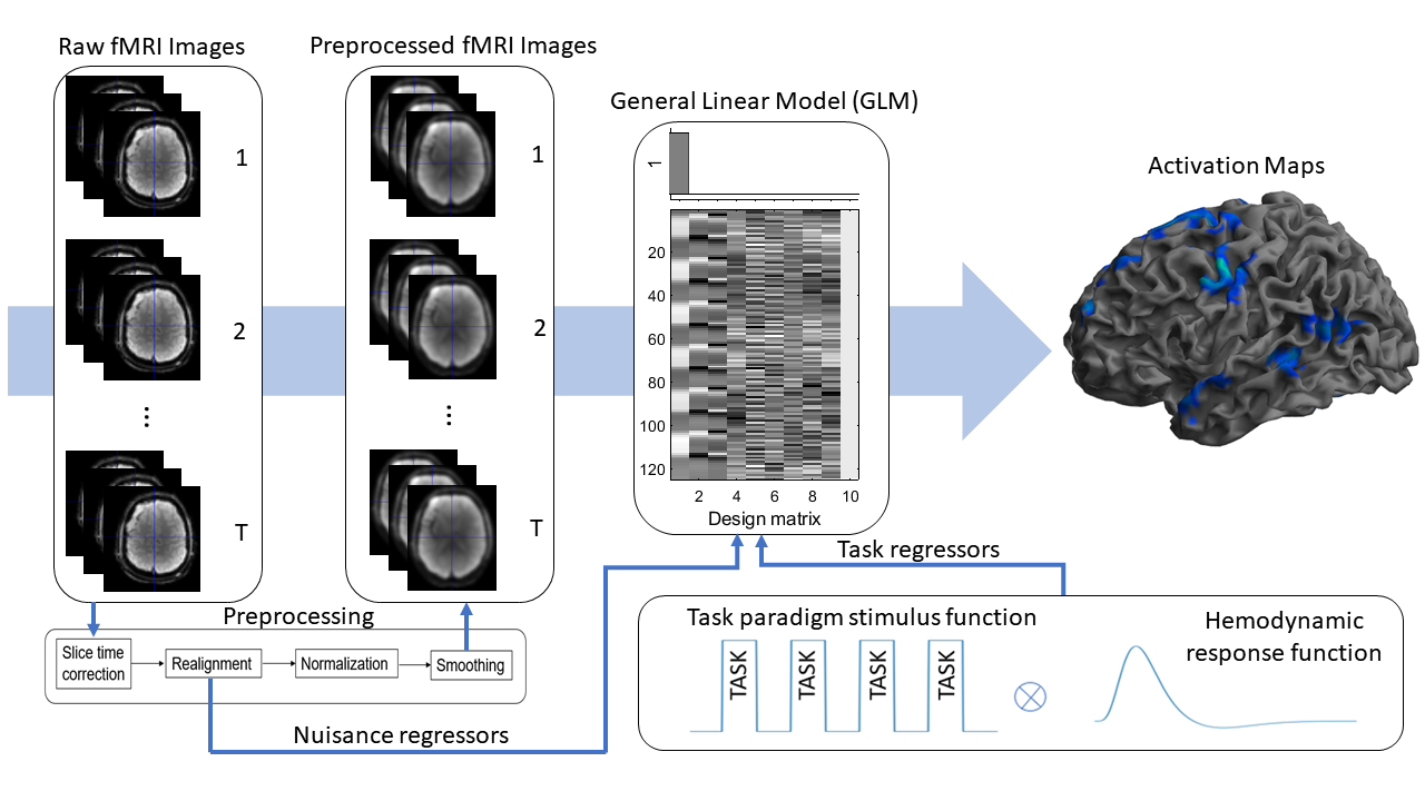
Figure 1. Illustrated are the
steps to obtain SPM12 activation maps. Task paradigm stimulus function was
convolved with the hemodynamic response function to get task regressors. Raw
fMRI images were preprocessed, and together with task and nuisance regressors
activation maps are produced using GLM modelling.
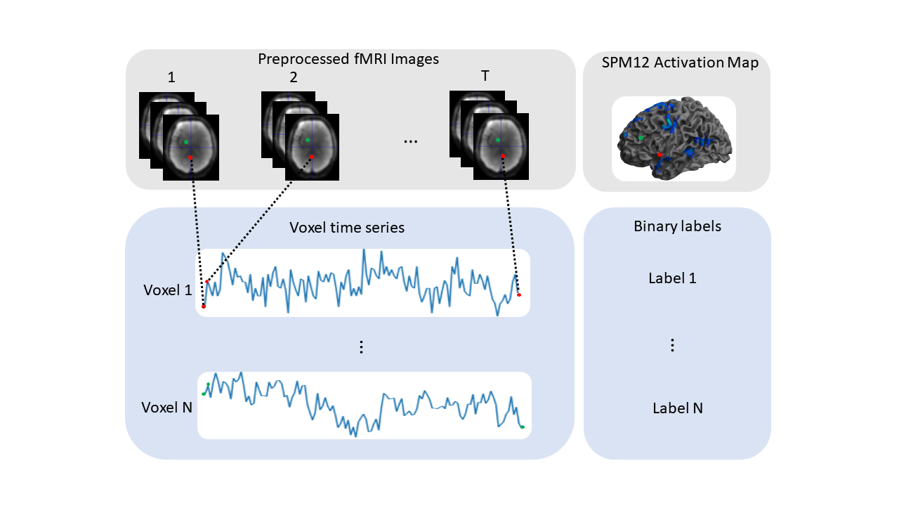
Figure 2. Illustrated are the
steps to extract voxel time series data and corresponding binary labels. SPM12
activation maps were used to define the 0 and 1 labels.
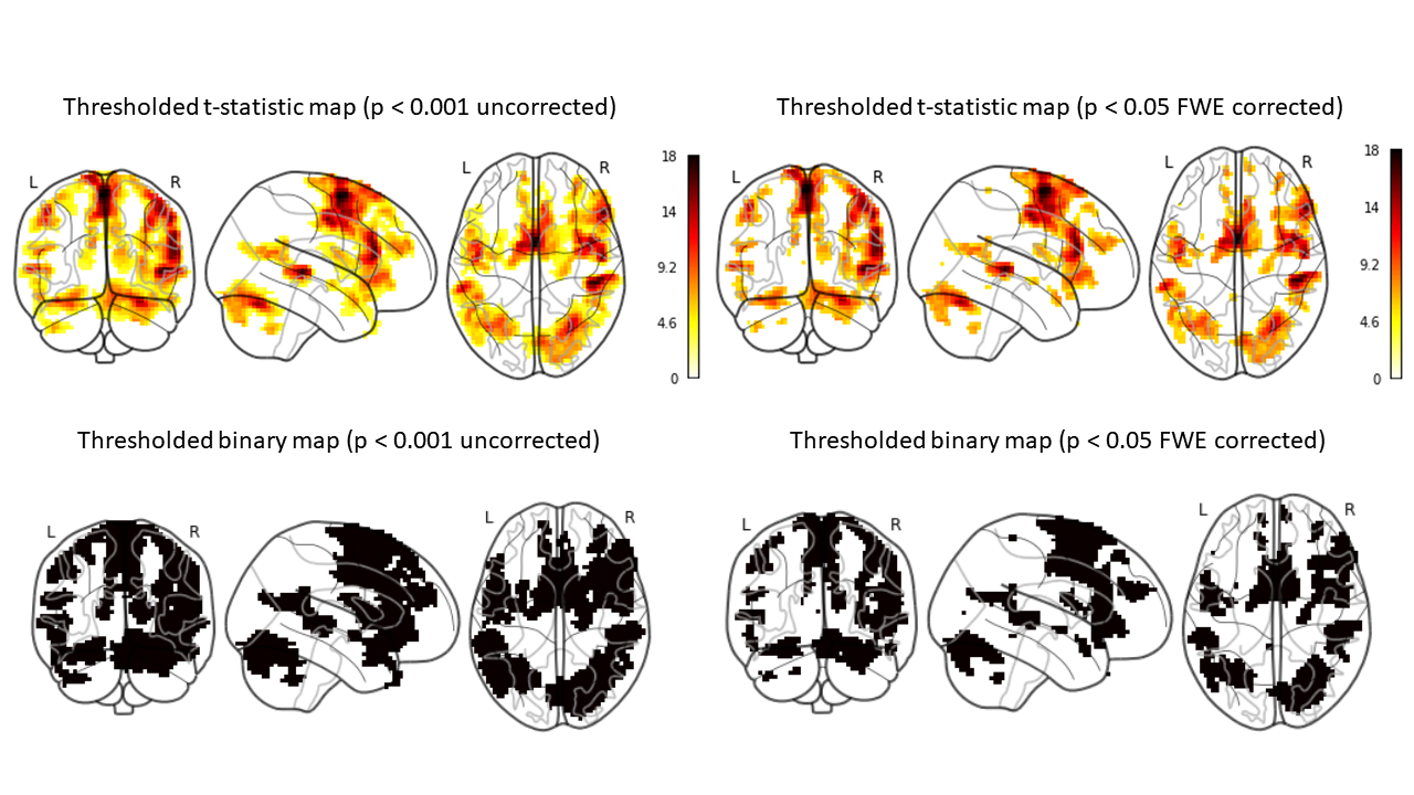
Figure 3. The SPM12 activation
maps based on different p-value thresholds (darker areas indicate a higher
t-statistic value) and its associated binary map (black - activation or label
1, white - non-activation or label 0).
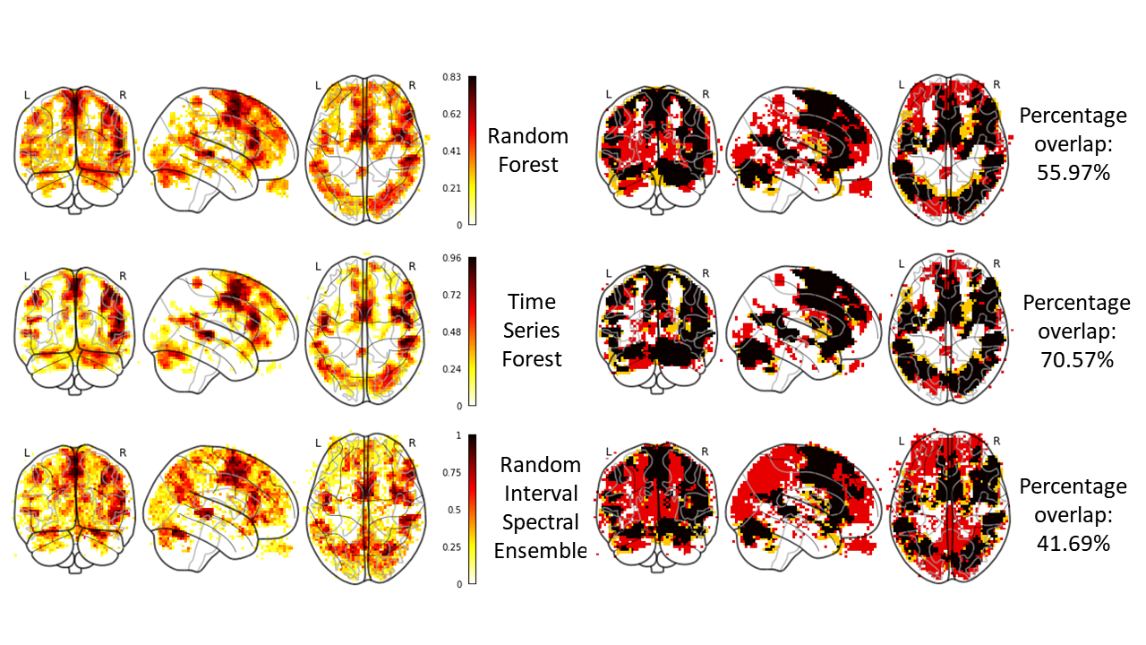
Figure 4. The images on the left
show the probability maps of three different models trained using SPM12
activation maps with threshold of p < 0.001 uncorrected (darker areas
indicate higher probability scores). The images on the right show
correspondence between the SPM12 activation map and the machine learning
prediction (black - area of overlap, yellow - activation areas found by SPM12,
red - areas predicted by machine learning models).
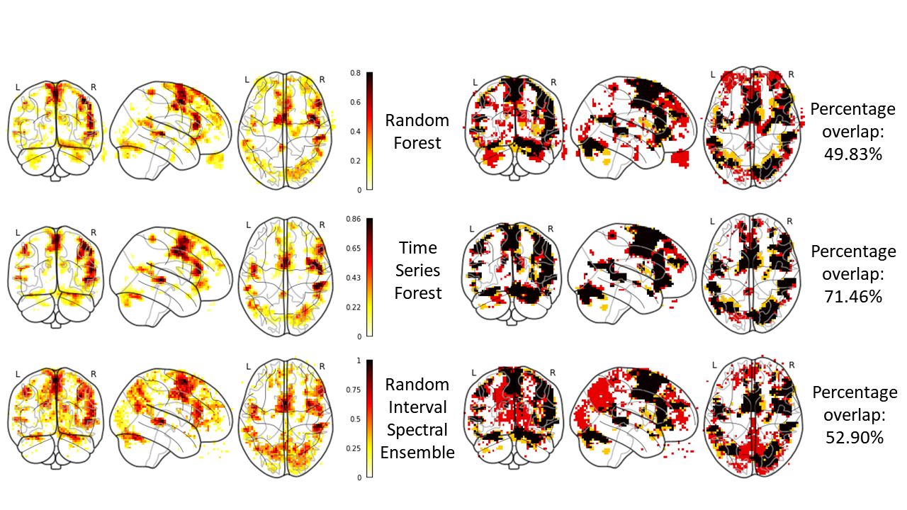
Figure 5. The images on the
left show the probability maps of three different models trained using SPM12
activation maps with threshold of p < 0.05 FWE corrected (darker areas
indicate higher probability scores). The images on the right show
correspondence between the SPM12 activation map and the machine learning
prediction (black - area of overlap, yellow - activation areas found by SPM12,
red - areas predicted by machine learning models).
DOI: https://doi.org/10.58530/2022/1909