1908
Full posterior estimation of Gray Matter cytoarchitecture using a three-compartment model with exchange: a simulation-based study1INRIA Saclay, Paris, France, 2INRIA Saclay, Palaiseau, France
Synopsis
We extract cytoarchitectural characteristics of brain gray matter from diffusion MRI signals including soma size, neurite signal fraction and water exchange. Our model improves on state-of-the-art in that 1) we extract an invertible system leading to stable parameters estimation, 2) our simulation-based inference approach allows to obtain the full posterior distribution of the parameters given a signal. Our solution is a two-step model. First, a new forward model relates summary statistics of the dMRI signal to different tissue parameters. Then, a likelihood-free inference-based algorithm is applied to invert the model, and returns a full posterior distribution over the parameter space.
Introduction
The characteristics of Gray Matter (GM) including water exchange is yet an unresolved problem in diffusion MRI (dMRI). However, as illustrated in figure 2, water exchange has a significant impact on the signal (up to a variation of 60%). Current exchange methods are considering models without soma, or propose unstable results5,6,7,8. We propose a new forward model that considers both water exchange and soma size, and which is invertible and more stable.Methods
Our work uses state of the art models6,7,8, where gray matter is modeled with three compartments, neurites (n), soma (s) and extra-cellular space (ECS), and accounts for exchanges between neurites and ECS. The proposed model estimates six key tissue parameters: the soma signal fraction fs, exchanging signal fractions of neurites and ECS fnex and fECSex, axial diffusivity inside the neurites Dn, a proxy to soma size1,5 Cs, and the exchange time tex. Diffusivity in the ECS is considered nearly constant for each subject, and estimated as 1/3 of the mean diffusivity in the ventricles9.Given an observation, we want to estimate the parameters $$$\theta = (f_{s}, f_{n}^{ex} , D_{n}, C_{s}, t_{ex})$$$ that produced it. In order to solve this inverse problem, we propose a two-fold analysis of the powder-averaged signal: one for small b-values and one for large b-values.
\begin{align*}
\left\{\begin{array}{l}
\left.\frac{\bar{S}(b)}{S(0)}\right|_{b\rightarrow 0} = \exp(-b\widetilde{D} -\frac 1 6 {b^2 \widetilde{D}^2 \widetilde{K}} +O\left(\frac{1}{b^{3}}\right))&\\
\left.\frac{\bar{S}(b)}{S(0)}\right|_{b\rightarrow\infty} = \sqrt{\frac{\pi}{4}}\frac{(1-f_{s})f_{n}^{ex}}{\sqrt{bD_{n}}}\exp{\left[-f_{ECS}^{ex}\left(\frac{t}{t_{ex}}\right)\right]}\left[1 + \frac{2f_{ECS}^{ex}\left(\frac{t}{t_{ex}}\right) + f_{n}^{ex}f_{ECS}^{ex}\left(\frac{t}{t_{ex}}\right)^{2}}{bD_{ECS}} + O\left(\frac{1}{b^{2}}\right)\right] \\
+ \exp{\left[-f_{n}^{ex}\left(\frac{t}{t_{ex}}\right)\right]}(1-f_{s})f_{ECS}^{ex}\left[1 - \frac{2f_{n}^{ex}\left(\frac{t}{t_{ex}}\right) + f_{n}^{ex}f_{ECS}^{ex} \left(\frac{t}{t_{ex}}\right)^{2}}{bD_{ECS}} +O\left(\frac{1}{b^{2}}\right) \right]\exp{\left(-bD_{ECS}\right)} \\
+ f_{s}\exp{\left[-\frac{\widetilde{C}_{s}}{\left(2\pi\right)^{2}t}b^{2}\right]}
\end{array}\right. \,
\end{align*}
The formula for small b-values is a cumulant decompostion of the powder-averaged signal, and a solution has been extended from 3,6. The large b-values approximation is more complex to invert. Therefore, we introduced a "truncated RTOP" for large b-values. By using the numerical-stability of the integral operator, we get a polynomial function of $$$q$$$ and $$$\log{q}$$$ that is easier to fit:
\begin{equation}
\left. RTOP(q_{min},q)\right|_{q_{min},q\rightarrow\infty} = 4\pi\int_{q_{min}}^{q} \left.\frac{\bar{S}(\eta)}{S(0)}\right|_{b\rightarrow\infty}\eta^{2} d\eta = a_{fit} + b_{fit}q^{2} + c_{fit}\log{q}
\end{equation}
We end up with a system of 6 equations, for 6 parameters:
\begin{align*}
\left\{\begin{array}{l}
\widetilde{D} =f_{s}\frac{C_{s}}{\left(2\pi\right)^{2}t} + \left(1-f_{s}\right)\bar{D}\\ \widetilde{K} = 3\frac{\left(1-f_{s}\right)}{\widetilde{D}^{2}}\left[f_{s}\left(\bar{D} - \frac{C_{s}}{\left(2\pi\right)^{2}t}\right)^{2} + \frac{\bar{D}^{2}\bar{K}}{3} \right]\\ a_{fit} = f_{s}\left[\left(\frac{\pi}{C_{s}}\right)^{\frac{3}{2}}erfc\left(\sqrt{C_{s}}q_{min}\right) + 2\pi q_{min}\frac{e^{-C_{s}q_min^{2}}}{C_{s}}\right] \\ - (1-f_{s})f_{n}^{ex}e^{-f_{ECS}^{ex}\frac{t}{t_{ex}}}\sqrt{\frac{\pi}{tD_{n}}}\left[\frac{q_{min}^{2}}{2} + \frac{\eta_{ex}}{\left(2\pi\right)^{2}tD_{ECS}}\log(q_{min})\right]\\ + (1-f_{s})f_{ECS}^{ex}e^{-f_{n}^{ex}\frac{t}{t_{ex}}}\left[\frac{1}{\left(4\pi tD_{ECS}\right)^{\frac{3}{2}}}\left(1-2\widetilde{\eta}_{ex}\right) + \frac{q_{min}e^{-\left(2\pi\right)^{2}tD_{ECS}q_{min}^{2}}}{2\pi tD_{ECS}}\right]\\ b_{fit} = (1-f_{s})f_{n}^{ex}e^{-f_{ECS}^{ex}\frac{t}{t_{ex}}}\sqrt{\frac{\pi}{4 tD_{n}}} \\ c_{fit} = (1-f_{s})f_{n}^{ex}e^{-f_{ECS}^{ex}\frac{t}{t_{ex}}}\sqrt{\frac{\pi}{ tD_{n}}}\frac{\eta_{ex}}{\left(2\pi\right)^{2}tD_{ECS}}\\ f_{n}^{ex} + f_{ECS}^{ex} = 1
\end{array}\right. \,
\end{align*}
Where $$$\eta_{ex} = 2f_{ECS}^{ex}\frac{t}{t_{ex}} + f_{n}^{ex}f_{ECS}^{ex}(\frac{t}{t_{ex}})^2$$$ and $$$\widetilde{\eta}_{ex} = 2f_{n}^{ex}\frac{t}{t_{ex}} + f_{n}^{ex}f_{ECS}^{ex}(\frac{t}{t_{ex}})^2$$$.
We solve this inverse problem using a likelihood-free inference algorithm2,4,5, which outputs the full posterior distribution of $$$\theta$$$ over the parameters space for a given observation.
We investigated the utility of the introduced summary statistics by comparing the posterior distributions obtained when directly fitting the powder-averaged signal, as done in 7, and when using summary statistics. Two exchange cases have been considered: first, we considered a small tex of 10ms, i.e. a high exchange rate between the neurites and ECS compartments, and then a high tex of 60ms, where the influence of exchanges can be considered negligible on the signal (Figure 2).
Results and Discussion
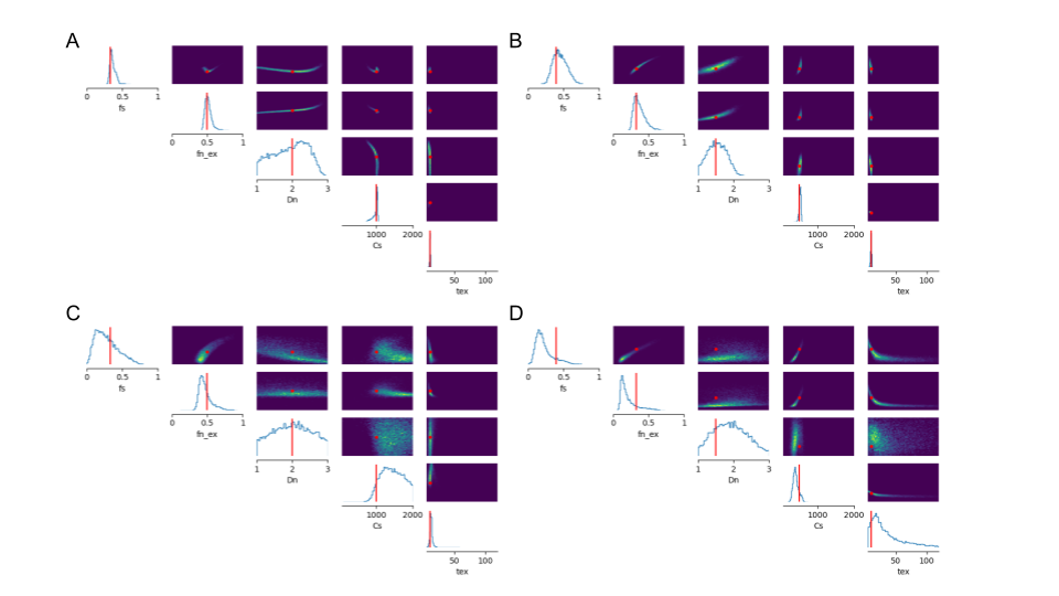
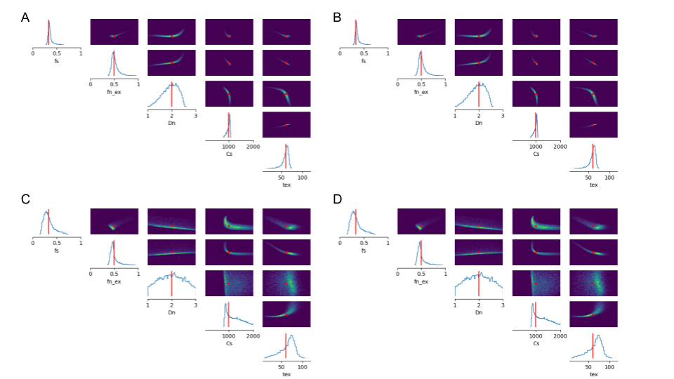
Two sets of $$$\theta$$$ have been considered in the simulations, both with tex = 10ms, 60ms: $$$\theta_{1} = (0.33, 0.5 , 2μm^{2}/ms, 1000μm^{2}, t_{ex})$$$ and $$$\theta_{2} = (0.4, 0.33, 1.5μm^{2}/ms, 500μm^{2},t_{ex})$$$, which correspond to spheres with radius rs = 16.7μm and 10.8μm and diffusivity Ds = 3μm2/ms. Figures 3 and 4, plots A and B, show the capacity of our model to estimate the tissue parameters from the summary statistics with good confidence. Exchanges between the neurites and ECS seem to influence the estimation of Dn, whose posterior distribution is wider for high exchanges.In comparison, the direct estimation from the powder-averaged signal indicates large indeterminacy regions, as can be seen in the joint posterior distributions of figures 3 and 4, plots C and D. This indeterminacy means that multiple $$$\theta$$$ can produce similar observed diffusion signal. Using summary statistics instead allows to greatly improve the robustness of the tissue parameters estimation.
Conclusion
Likelihood-free inference methods allow to estimate the full posterior distribution of the tissue parameters and therefore uncover indeterminacy areas. Applying this method directly to powder-averaged signals showed the instability of the fitting of the parameters in that case. We propose to use summary statistics extracted from a low and high b-values analysis instead, which greatly reduce the indeterminacy regions.Acknowledgements
This work was supported by the ERC-StG NeuroLang grant number 757672 and the ANR/NSF NeuroRef grants.References
1. Balinov B., Jonsson B., Linse P., Soderman O. .The NMR Self-Diffusion Method Applied to Restricted Diffusion. Simulation of Echo Attenuation from Molecules in Spheres and between Planes. 1993
2. Cranmer, K., Brehmer, J., Louppe, G.: The frontier of simulation-based inference.Proceedings of the National Academy ofSciences117(48), 30055–30062 (2020)
3. Els Fieremans, Dmitry S Novikov, Jens H Jensen, Joseph A Helpern. Monte Carlo study of a two-compartment exchange model of diffusion. 2010.
4. Greenberg, D., Nonnenmacher, M., Macke, J.: Automatic posterior transformationfor likelihood-free inference. In: Proceedings ofthe 36th International Conference onMachine Learning, vol. 97, pp. 2404–2414, PMLR (2019)
5. Maëliss Jallais, Pedro Luiz Coelho Rodrigues, Alexandre Gramfort, Demian Wassermann. Cytoarchitecture Measurements in Brain Gray Matter using Likelihood-Free Inference. 2021.
6. leana O. Jelescu, Alexandre de Skowronski, Marco Palombo, Dmitry S. Novikov. Neurite ExchangeImaging (NEXI): A minimal model of diffusion in gray matter with intercompartment water exchange. 2021.
7. Jonas L. Olesen, Leif Østergaard, Noam Shemesh, Sune N. Jespersen. Diffusion time dependence,power-law scaling, and exchange in gray matter. 2021.
8. Marco Palombo, Andrada Ianus, Michele Guerreri, Daniel Nunes, Daniel C. Alexander, Noam Shemesh,Hui Zhang. SANDI: A compartment-based model for non-invasive apparent soma and neurite imagingby diffusion MRI. 2020.
9. Vincent, Mélissa and Gaudin, Mylène and Lucas-Torres, Covadonga and Wong, Alan and Es-cartin, Carole and Valette, Julien.Characterizing extracellular diffusion properties using diffusion-weighted MRS of sucrose injected in mouse brain, NMR in Biomedicine, 34, 4, e4478, 2021.https://doi.org/10.1002/nbm.4478
Figures
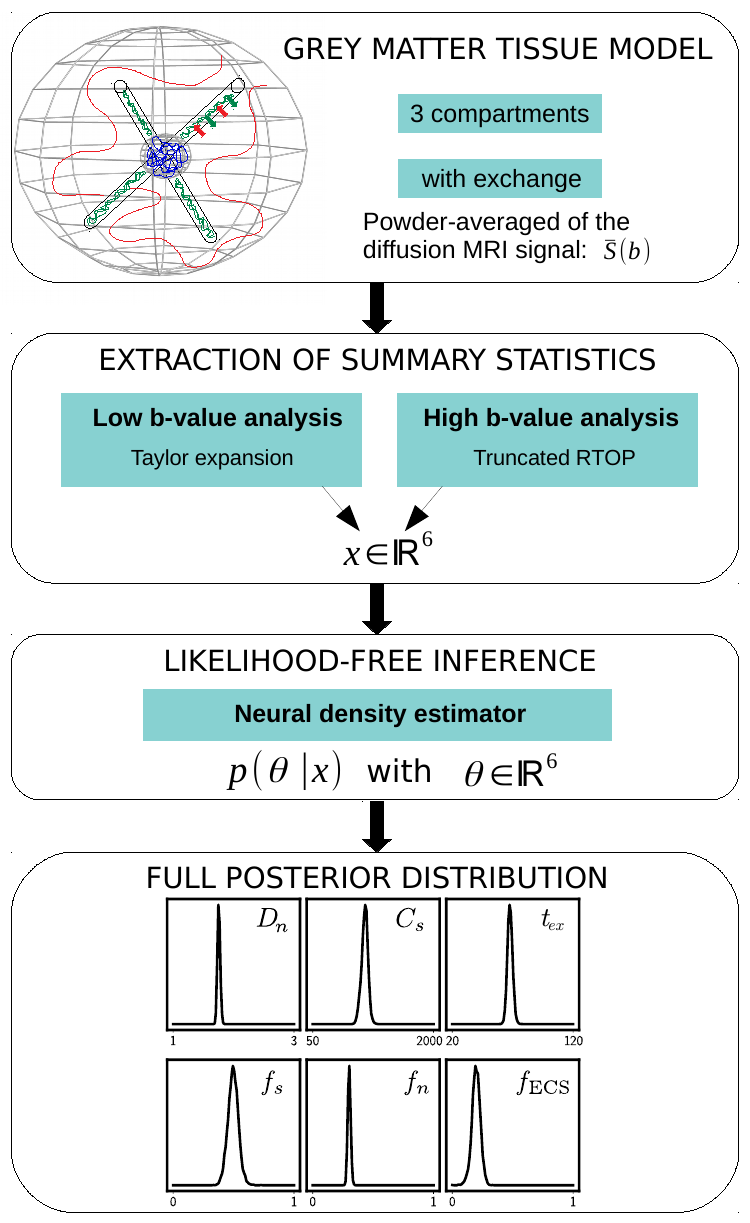
Figure 1 - Visual abstract. We start by modeling brain gray matter with three compartments: somas, neurites and extra-cellular space, with exchange between neurites and the ECS. We then extract summary statistics from the powder-averaged signal using a low and high b-values analysis. Applying a likelihood-free inference algorithm allows to estimate both the parameters and their full posterior distribution.
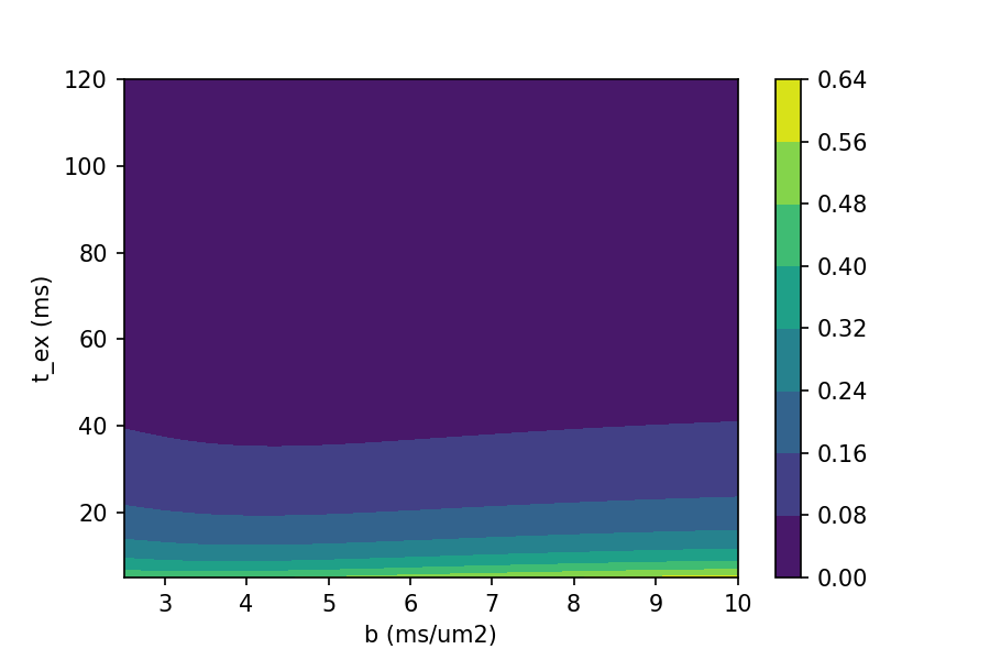
Figure 2 -Relative variation of the powder-averaged signal with regard to the direction-averaged signal computed for tex = 120ms. Exchanges are undetectable at such high diffusion exchange times, and this regime is close to the SANDI model6. A clear dependence of tex on the signal is observed, with a variation up to 64%.