1906
Using a Spherically Distributed Spirals Trajectory to Collect Coil Sensitivity Maps for Iterative SENSE Reconstruction1Radiology, Mayo Clinic, Rochester, MN, United States, 2MR R&D, Philips Healthcare, Rochester, MN, United States
Synopsis
Conventionally, Cartesian pre-scans are collected over several seconds to create accurate coil sensitivity maps (CSM) for SENSE reconstruction of under-sampled MRI data, with body-coil images used for signal normalization. Since body coils have a larger sensitivity region than phased-array coils, these pre-scans typically employ a very large field-of-view (FOV) to avoid aliasing, leading to low-resolution CSM and potential small errors in subsequent reconstructions. This abstract proposes a new CSM pre-scan sequence using a spherically-distributed-spirals trajectory. The acquisition efficiency and incoherent aliasing offered by this trajectory allow for smaller FOV and higher resolution while maintaining similar scanning time as conventional pre-scans.
Introduction
For successful implementations of parallel imaging techniques such as SENSE1 on under-sampled MRI data, prior knowledge about the sensitivities of coil elements is needed to disentangle the aliased images2. On clinical scanners, this is typically done during pre-scan by running a Cartesian low-resolution sequence with both body and phased-array coils to obtain coil sensitivity maps (CSM). However, due to the constraint on acquisition time (a few seconds) and the need for a large field of view (FOV) to avoid folding artifacts due to signal from outside of FOV in certain scenarios (such as the presence of an I.V. line), the voxel size is kept very large, and the resulting CSM is cropped and interpolated to match the FOV and resolution of following imaging sequences. The Spherically Distributed Spirals (SDS) trajectory3 efficiently collects data in a 3D spherical volume in k-space using golden-angle rotation4 of a single spiral waveform about a common axis. Consequently, folding caused by signal from outside of FOV is highly incoherent among spiral arms and is dispersed across the final images. In this study, we take advantage of these characteristics to design a pre-scan sequence that can be used to acquire higher-resolution CSM data without an increase in scan time. Results suggest the method is robust to the presence of signal from outside of the acquired FOV.Methods
Data AcquisitionBrain experiments were conducted on a 1.5T scanner (Ambition, Philips Healthcare, Best, Netherland) with institutional IRB approval and written informed consent from healthy subjects using a 15-channel head and neck surface phased-array coil. To assess the effects of signal outside of the FOV, a 10-cc syringe filled with water doped with copper sulfate was placed above the eyes of the subject outside of the phased-array coil (Fig. 1). Low-resolution CSM data were acquired using an SDS gradient-echo sequence with spiral-out readout in 7s (FOV=270mm3, resolution 4.22mm3, TE=4.6ms, TR=12.4ms, flip angle=6.7°, readout=5.7ms, 420 total encoding steps) with both surface and body coils to match the scanning time of an optimized Cartesian pre-scan (FOV=700mm2, resolution=11.2mm2, 94 slices, slice thickness 11mm, slice gap -5.5mm). Fully-sampled high-resolution images were acquired using a spiral-out stack-of-spirals (SOS) gradient-echo sequence in 3min20sec (FOV=230mm2×150mm, resolution 0.7mm2×2mm, TE=2.3 and 4.6ms, TR=24ms, flip angle=27.9°, readout=14.5ms, 6 arms per slice) using surface coils only. A larger FOV was prescribed for SDS to accommodate for the sizes of different subjects that may be encountered in a pre-scan.
CSM Calculation and Coil Combination
Fig. 2 shows the pipeline for CSM calculation. Magnitude and phase images from surface and body coils were separately smoothed by applying a 3D Gaussian filter with a 1.5-voxel standard deviation in the kernel to avoid phase cancellation and then linearly interpolated to match the matrix size of high-resolution images. For fully-sampled high-resolution data, coil-combined image I is calculated using $$$I=\frac{\Sigma_i(C_i\cdot\lambda_i^{-1})\cdot I_i}{\Sigma_i(C_i\cdot C_i^*)}$$$, where Ci is the CSM of coil i, Ii the image from coil i and λi the i-th diagonal element of the noise covariance matrix4. The high-resolution SOS k-space was also retroactively under-sampled by a factor of R=2, and coil-combined using iterative SENSE1.
Deblurring and fat/water separation5 were performed on coil-combined images with Cartesian B0 field maps acquired with a vendor-provided sequence.
SNR Calculation
Two sets of under-sampled images were reconstructed from each half of k-space and relative SNR was calculated voxel-wise as the ratio of their mean to standard deviation. Six regions of interest (ROI) of 50 pixels in size were drawn in two slices inside the brain to calculate the mean SNR using each CSM.
Results and Discussions
Fig. 3 shows the comparison between the low-resolution CSM of all channels from the Cartesian and SDS pre-scans, where magnitude is represented by the brightness and phase by the color of each pixel. While both methods had generally similar CSM profiles, their ratio shows that Cartesian scan retained some contrast of the brain in the final CSM results, as highlighted by the red arrows. The greatest difference was observed around the nose as indicated by the white dashed boxes, where close-ups in the bottom row demonstrated that SDS was able to mitigate the signal cancellation observed in Cartesian CSM which possibly stemmed from imperfect interpolation between large voxels.Fig. 4 shows the deblurred water images in two slices, with the CSM of the bottom slice shown in Fig. 3. Compared to fully-sampled k-space, iterative SENSE of R=2 showed reduced SNR with both sets of CSM. The residues between fully- and under-sampled deblurred images after normalization are shown in the same sale and show that CSM from SDS pre-scan produced lower errors than Cartesian pre-scan around the nose, suggesting a more accurate CSM result by SDS pre-scan in that area.
Fig. 5 shows the relative SNR of under-sampled images, which averaged to 33.7a.u. and 34.8a.u. for Cartesian and SDS CSM respectively inside the six ROIs, suggesting similar SNR levels.
Conclusions
A spherically-distributed spirals trajectory was used to acquire high-resolution CSM within a few seconds with smaller FOV in presence of signal outside of the FOV. Volunteer brain studies showed SDS to have equivalent to slightly better performance than Cartesian pre-scan in under-sampled (R=2) dataset using iterative SENSE reconstruction.Acknowledgements
This work was partially funded by Philips Healthcare and supported by its MR R&D team in Rochester, MN USA.References
1. Pruessmann KP, Weiger M, Scheidegger MB et al. SENSE: sensitivity encoding for fast MRI. Magn Reson Med. 1999;42(5):952-962
2. Guo JY, Kholmovski EG, Zhang L et al. Evaluation of motion effects on parallel MR imaging with precalibration. Magn Reson Med. 2007;25(8):1130–1137
3. Turley DC, Pipe JG. Distributed spirals: a new class of three-dimensional k-space trajectories. Magn Reson Med. 2013;70(2):413-419
4. Winkelmann S, Schaeffter T, Koehler T et al. An optimal radial profile order based on the Golden Ratio for time-resolved MRI. IEEE Trans Med Imaging. 2007;26(1):68-76
5. Wang D, Zwart NR, Pipe JG. Joint water-fat separation and deblurring for spiral imaging. Magn Reson Med. 2018;79(6): 3218-3228
Figures

Figure 1: Sketch showing the experimental setup for acquisition of CSM in the head with water signal present outside of FOV.

Figure 2: Flow chart showing the calculation of CSM from low-resolution images.

Figure 3: The top row shows CSM results of all channels from the low-resolution Cartesian and SDS pre-scans, and the ratio between the two sets. The phase is encoded in the color of each pixel and represented by the pinwheel at the bottom right corner in all subfigures. The bottom row shows close-ups of white dashed boxes.
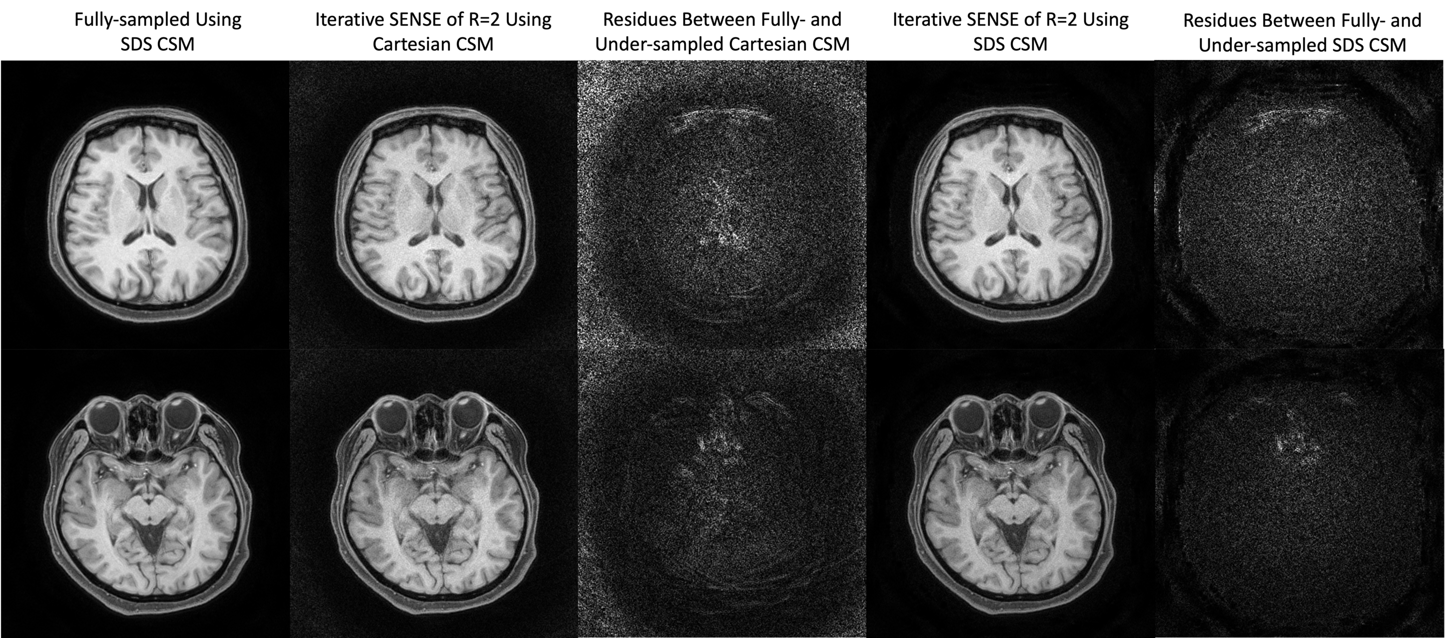
Figure 4: Two slices of deblurred water images using the fully-sampled k-space data (first column), retroactively undersampled k-space data using Cartesian pre-scan CSM (second column) and retroactively under-sampled k-space data using SDS pre-scan CSM (fourth column). The residues between the under-sampled and fully-sampled images after normalization are shown in the third and fifth columns for CSM from Cartesian and SDS pre-scans respectively.
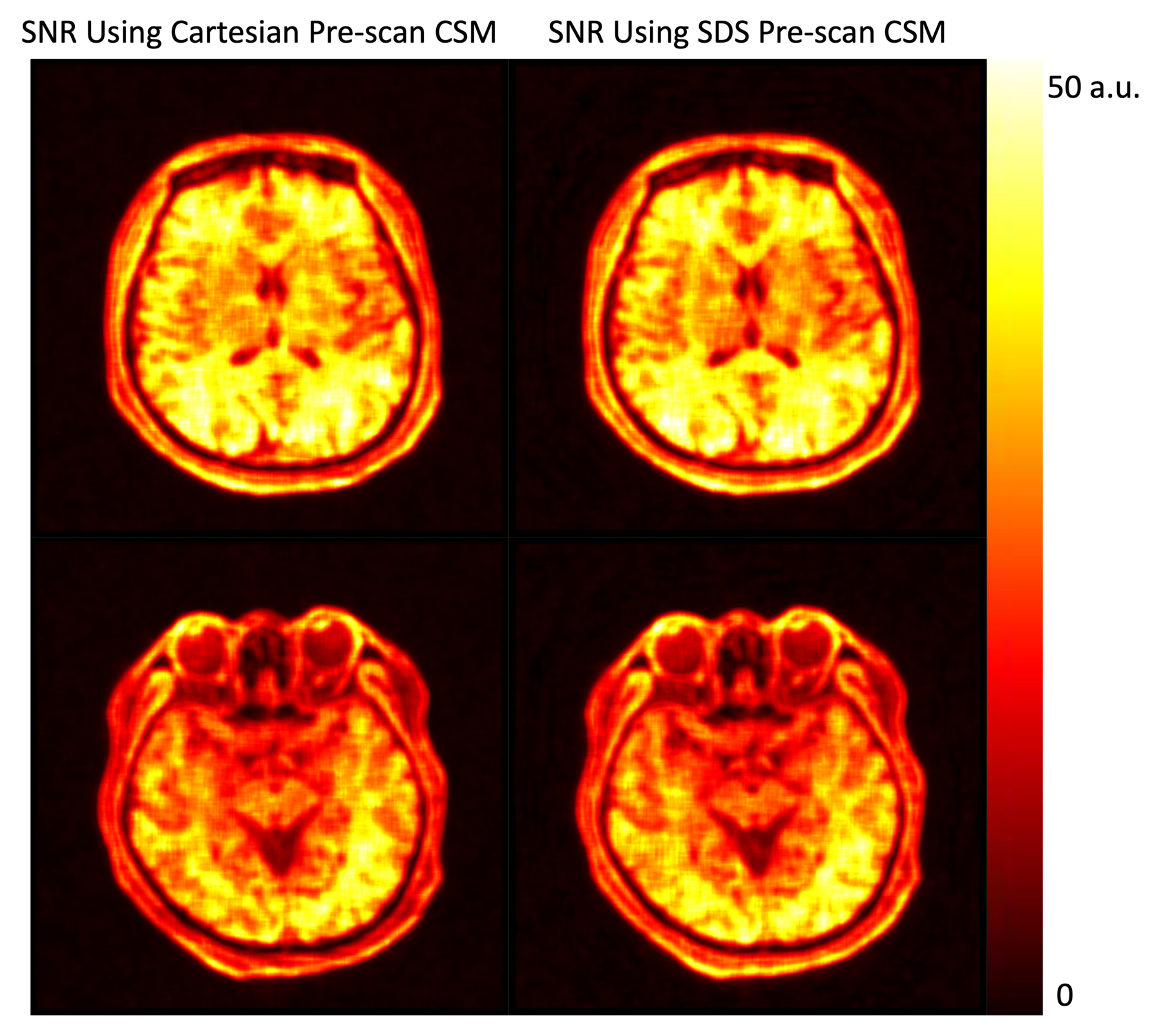
Figure 5: Relative SNR maps of SENSE reconstruction using CSM from Cartesian and SDS pre-scans.