1897
Simulated Impact of Gradient Amplifier Noise on Simple 3D Sequences: Preliminary Results1Hyperfine, Guilford, CT, United States
Synopsis
It is often stated, without qualification, that MRI gradient systems must be precise and/or accurate in order to ensure MRI image quality. Some imperfections (delay, eddy currents) have been well-studied and documented, while others such as noise, ripple, and quantization have not. Here we simulate the impact of white noise in the gradient fields with simple cartesian imaging sequences for a numerical brain phantom. Preliminary results suggest that high-performance/high-cost components typically marketed for gradient control are excessive, and much cheaper components could be used without significant drawbacks (NRMSE < 1%), especially for low-field/low-cost systems.
Background
The gradient system of a MRI scanner spatially encodes the position of spins by modulating phase and frequency, and thus the fidelity of the gradient system is critical for image quality. For the gradient system engineer, there are some specifications whose relationship to image quality are well-known. These include limits to maximum output and slew rate, as well as eddy currents and spatial linearity. However, there are numerous aspects of the gradient system, particularly the gradient power amplifier, which are not well-documented. These include stochastic effects such as amplifier noise (due to noise in current feedback sensors), quantization noise (from limited ADC and PWM resolution), and output ripple (for modern GPAs based on PWM). Various sources make broad claims about the noise/ripple specifications of GPAs, often suggesting the need for precision on the order of a few milliamps or ppm1–6, or that the required precision is simply high7–9, but without qualification. This author was unable to find any example of the impact of gradient noise/ripple on image quality. The purpose of this study is to provide some very preliminary examples of effects on simple imaging sequences.Methods
All simulations were carried out using MATLAB 2016 on the author’s personal desktop computer. The simulation architecture is described in figure 1. Up to four parameters could be swept in each experiment. Table 1 describes all the available parameters the experiment could vary. The simulation takes a sequence parameter set and creates ideal gradient G(t) and RF waveforms. The ideal sequence is used to create a reference image. This is then repeated ten times with white noise Gnoise(t) added to G(t), yielding ten corrupted images. Gnoise(t) is taken from a white noise dictionary, and the same ten noise seeds are always used, allowing for repeatable results. By default, Gnoise(t) had an amplitude spectral density of $$$\sqrt{\overline{g_n^2}}=40nT/m/\sqrt{Hz}$$$, approximately 100 times higher than fluxgate current transducers marketed for MRI applications9,10 (for a system Gmax of 40mT/m per axis). Anatomical brain phantoms from BrainWeb11 were used (discrete model, subject 04). Only T1, T2, and M0 were included in the simulations (B0 and B1 were assumed to be homogeneous). The images are reconstructed with a simple IFFT. Image corruption is measured by normalized RMSE as defined below, where $$$x$$$ is the reference image and $$$x^*$$$ is a corrupted image.$$NRMSE=\frac{\sum_i^N|x_{i}-x_i^*|^{2}}{\sum_i^N|x_{i}|^{2}}$$
Results
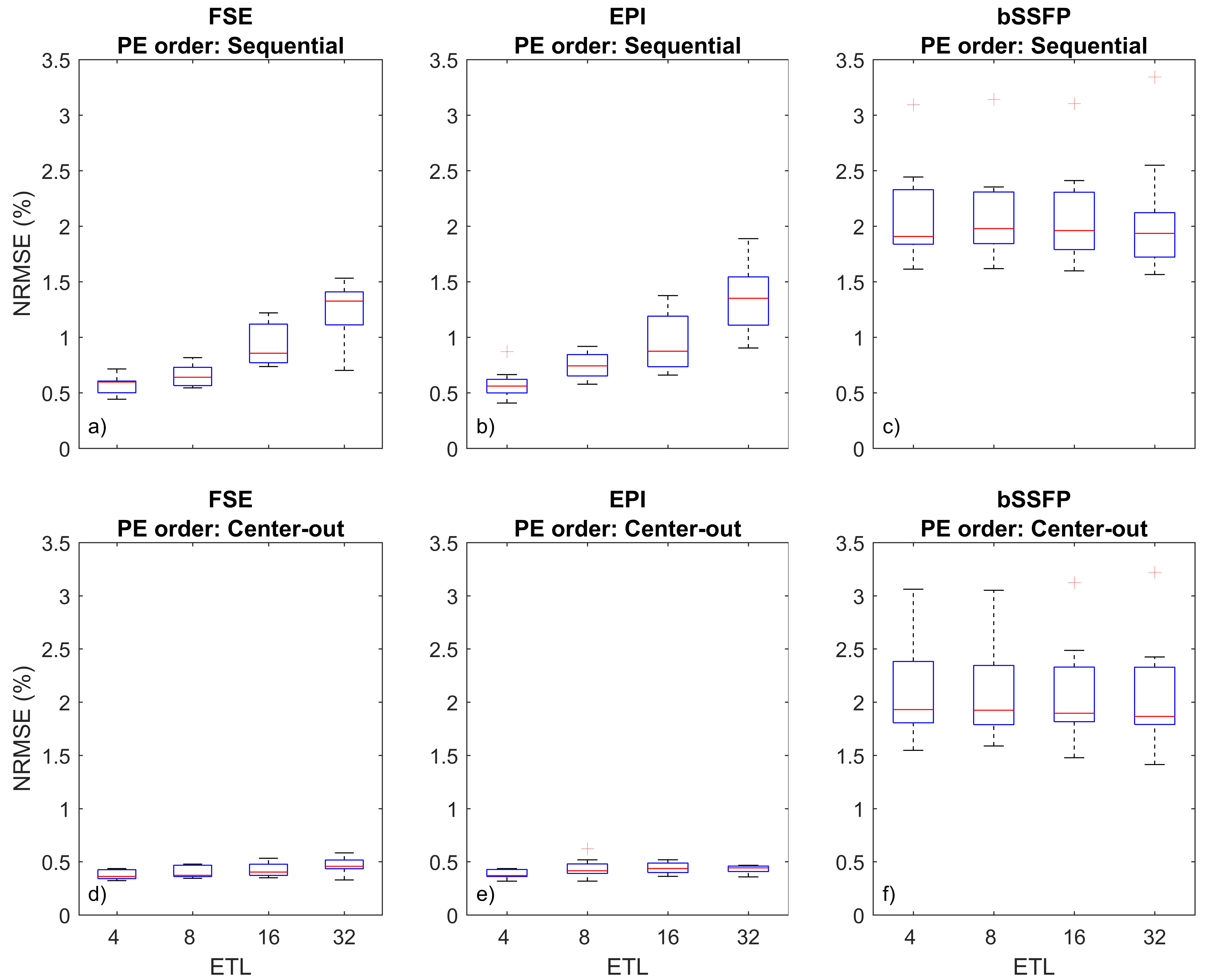
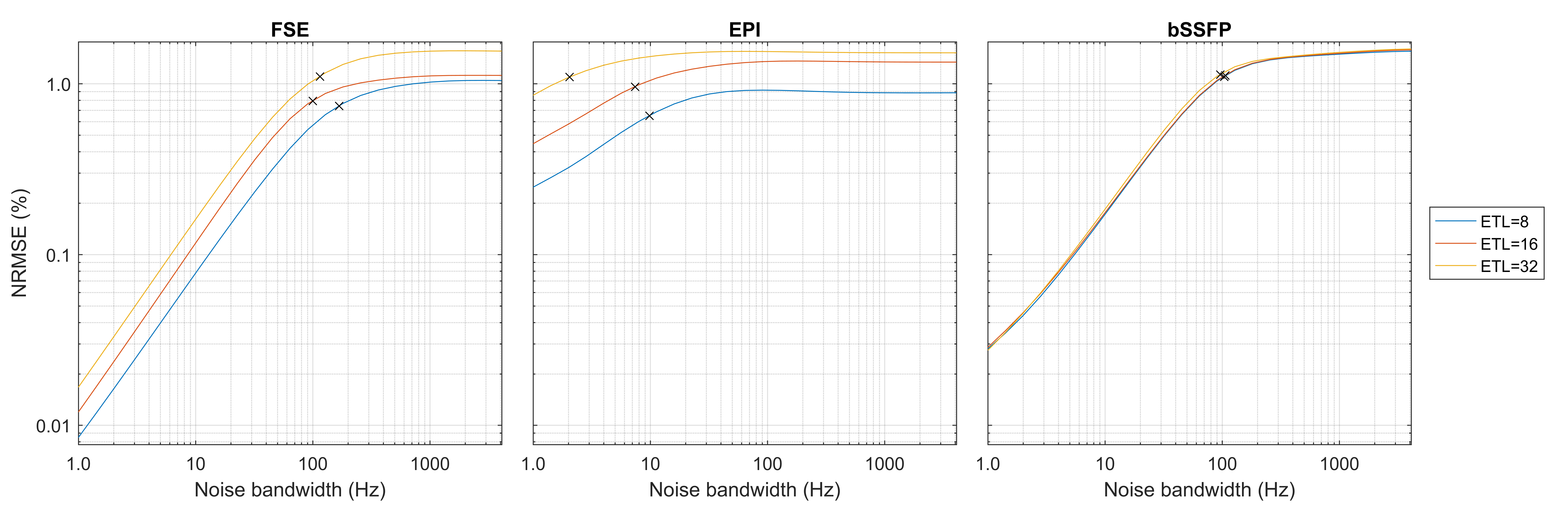
Two particular experiments were selected for this abstract. Table 1 shows the parameters used for each experiment. Experiment 1 demonstrates the impact of basic sequence parameters on Gnoise-induced error. Figure 2 shows a subset of the resulting image artifacts. Figure 3 shows a more complete summary of the dataset (see captions for explanation).In experiment 2, Gnoise(t) was passed through a first order lowpass filter to limit noise bandwidth BWnoise to between 1Hz and 4.096kHz. ETL also varied (8, 16, and 32). Figure 4 shows mean NRMSE vs BWnoise for different sequences. For all three sequence types, mean NRMSE increases with BWnoise until some corner frequency fc. For FSE and bSSFP, fc was near 100Hz, likely related to the echo spacing of 5ms. For EPI, fc was 2-10Hz, depending on the ETL.
Discussion
Artifacts appeared as random ghosting in the PE direction(s), similar to motion artifacts. For EPI and FSE, NRMSE increased with effective TE, and thus T2 weighted sequences were much more susceptible to Gnoise(t). For bSSFP, encoding order had no obvious impact on NRMSE; cumulative phase errors are expected to increase for longer relaxation times. The highest observed NRMSE was 3.34% for bSSFP with ETL=4.Experiment 2 showed that noise content above 1/ESP had little impact on NRMSE. Furthermore, the refocusing pulses in FSE and bSSFP were effective at rejecting lower frequency noise. Further simulations (not shown) show this becomes particularly relevant when adding 1/f noise. However, it seemed that FSE and bSSFP were particularly susceptible to noise with frequency content near 1/ESP.
Further simulations (not shown here) showed that NRMSE did not depend strongly on voxel size (kmax), but did trend strongly with FOV (1/Δk). It was also found that NRMSE scaled very linearly with noise density $$$\sqrt{\overline{g_n^2}}$$$. Scaling Gnoise down to the level expected for ultrastable current transducers ($$$\sqrt{\overline{g_n^2}}=0.4nT/m/\sqrt{Hz}$$$ for Gmax=40mT/m) would thus yield a worst-case NRMSE of only 0.0334% for the same sequence parameters. For high-field MRI systems, such overspecced hardware is generally the norm, and makes little difference in the total bill of materials. But for development of low-field/low-cost MRI systems, forgoeing such excesses may significantly reduce costs without compromising image quality.
Yet it must be emphasized that this study represents a tiny fraction of the degrees of freedom available to sequence designers. For example, parallel imaging, phase-contrast imaging, and non-cartesian trajectories may be much more susceptible to Gnoise than shown here. Such topics, along with other Gnoise types (PWM ripple and quantization noise) will be considered in future work.
Acknowledgements
No acknowledgement found.References
[1] “ADI’s Magnetic Resonance Imaging (MRI) Solutions.” Analog Devices, 2013.
[2] Scarlett J. “Advancements in MRI Architectures Reduce Design Complexity While Improving Image Quality.” EETimes, 2010.
[3] Schmitt F, Nowak S, Eberlein E. “An Attempt to Reconstruct the History of Gradient-System Technology at Siemens,” 2020.
[4] Pachchigar M. “High-Performance Data-Acquisition System Enhances Images for Digital X-Ray and MRI.” Analog Devices, 2013.
[5] Sabate J et al. “Ripple cancellation filter for magnetic resonance imaging gradient amplifiers.” IEEE APEC, 2004.
[6] Webb A. “Magnetic resonance technology: hardware and system component design.” Cambridge, UK: Royal Society of Chemistry; 2016.
[7] Wang R et al. “High efficiency power converter with SiC power MOSFETs for pulsed power applications,” IEEE ECCE, 2017.
[8] Sabate J et al. “Magnetic Resonance Imaging Power: High-Performance MVA Gradient Drivers.” IEEE JESTPE, 2016.
[9] “High Precision Current Transducers.” LEM USA. https://www.lem.com/en/file/5619/download
[10] “Ultra-Stable & High Precision Current Transducers.” Danisense, 2018. http://www.danisense.com/images/pdf/selectionGuide/Shortform.pdf
[11] Cocosco C et al. “BrainWeb: Simulated Brain Database.” https://brainweb.bic.mni.mcgill.ca/brainweb/faq.html
[12] Hargreaves B. “Bloch Equation Simulator.” 2003. http://mrsrl.stanford.edu/~brian/blochsim/
Figures
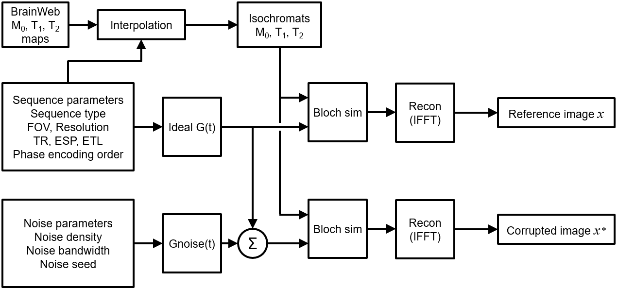
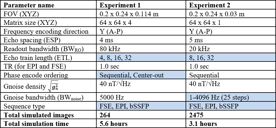
Table 1. Summary of parameters used in both experiments. Swept parameters are highlighted in blue. For each parameter combination, eleven images were simulated, one being the uncorrupted reference image and ten being corrupted by Gnoise(t).