1846
Combining machine learning and mathematical modeling in estimation of T1 relaxation time1Department of Mathematics, FNSPE CTU in Prague, Prague, Czech Republic, 2Department of Radiology, Institute for clinical and experimental medicine, Prague, Czech Republic, 3Artificial Intelligence Center, CTU in Prague, Prague, Czech Republic, 4Department of Pediatrics, UT Southwestern Medical Center, Dallas, TX, United States
Synopsis
A method for estimating tissue parameters using cardiovascular MRI and biophysical model by combining neural network (NN) and numerical optimization (NO) is illustrated on estimating $$$T_1$$$ relaxation time from MOLLI. Compared to the estimation obtained from MOLLI by the scanner, the proposed method provided $$$T_1$$$ closer to turbo spin-echo pseudo-ground in 7 out of 8 phantoms and higher or comparable myocardial and blood $$$T_1$$$ in 6 out of 7 patiens’ datasets. Including the NN-based initial guess accelerated the subsequent NO. NO initialized by NN, trained using simulated data, showed the potential to increase the efficiency and robustness of parameter estimation.
Introduction
Both mathematical models and machine learning (ML) methods can be used to enhance medical measurements. Fully biophysical models allow estimating material parameters that represent the physical properties of the tissue (e.g. passive myocardial stiffness and contractility using cine or tagged MRI (1;2)). In this work, we propose a two-stage parameter estimation method, which combines ML, mathematical model, and numerical optimization. The proposed method is illustrated on the problem of estimating the $$$T_1$$$ relaxation time from image series acquired by the Modified Look-LockerInversion recovery technique (MOLLI) (3). The process of longitudinal tissue relaxation can be described by a phenomenological model of an exponential function with the time constant $$$T_1$$$. Alternatively, a biophysical approach, typically using a mathematical model of the relaxation process described by Bloch equations – a Bloch simulator (4) – can be employed. Recently, both ML (5) and numerical optimization (6) were used to estimate the parameters of the Bloch simulator. In the present work, we combine these approaches to benefit from both. In the first stage, the mathematical model of the MOLLI sequence is used to generate a training dataset for NN, which can produce a fast initial guess of the parameters. In the second stage, the actual parameters of the given measurement are substituted into the mathematical model of MOLLI. This “patient and measurement-specific” model is then used to fine-tune the NN estimate by numerical optimization.Methods
We use a mathematical model of the MOLLI sequence $$$F(\vec{q})$$$, where $$$\vec q$$$ are parameters of the imaging sequence and the imaged tissue, i.a. $$$T_1$$$, and the output is a vector of generated intensities of the given pixel, see schematics in Figure 1. The $$$T_1$$$ estimation is formulated as an inversion problem.In the first stage, the initial estimation of the tissue parameters $$$\vec{p}=(T_1,T_2,M_0)$$$ is obtained from the NN. For the range of model parameters used in the training phase, see Table 2.
For the second stage, the model $$$F$$$ is turned into the "patient- and measurement-specific" model $$$\tilde{F}$$$ by inputting the parameter values from the DICOM header. Then, the remained free parameters $$$T_1,T_2,M_0$$$ are optimized to minimize the difference between the measured and generated signal:
$$\min_{T_1,T_2,M_0}l(\tilde{F}(T_1,T_2,M_0),\vec{ s}).$$
To deal with the ill-posedness of this problem, the loss function
$$l(\vec{s},\tilde{\vec s})=0.05\left(\sum_{i=1}^2(s_i-\tilde{s}_i)^2+\sum_{i=7}^{11}(s_i-\tilde{s}_i)^2 \right)+\sum_{i=3}^6(s_i-\tilde{s}_i)^2$$
assigns lower weights to signals sampled at the end of the relaxation curve, that are primarily affected by $$$M_0$$$ and less by $$$T_1$$$ and higher weights to sampling points in which the relaxation curve grows steeply and are primarily affected by the $$$T_1$$$.
The variational formulation of the second stage allows to include additional constraints. In our illustrative example, it is a term ensuring the smoothness of the parameter maps.
The proposed method was validated on eight phantoms imaged on a 3T MRI scanner. Results of the proposed approach were compared with the $$$T_1$$$ estimation from the same MOLLI dataset provided directly by the scanner console $$$T_1^{scanner}$$$ against pseudo-ground truth values obtained by the inversion recovery turbo spin-echo (IR-TSE) $$$T_1^{GT}$$$.
The estimations were also compared on datasets of seven patients indicated for a CMR exam. The datasets were acquired under the ethical approval number G-14-08-11, in conformance with the 1975 Declaration of Helsinki, on a 1.5T MRI scanner.
Results
We denote: $$$T_1^{NN}$$$ the initial estimate obtained by NN; $$$T_1^{NN,NO}$$$ the result of the numerical optimization initialized by NN. $$$T_1^{NN,NO}$$$ was closer to $$$T_1^{GT}$$$ in 7 out of 8 phantoms, see Table 3. The second stage provided more even results, compared to NN – while the percentage error with respect to $$$T_1^{GT}$$$ varied between -19.42 and 8.57% for the NN-estimation, it was improved to 1.97-10.17% after NO. Contrary to $$$T_1^{scanner}$$$, the percentage error of $$$T_1^{NN,NO}$$$ does not increase with increasing $$$T_1$$$.In the in vivo data, $$$T_1^{scanner}$$$ and $$$T_1^{NN, NO}$$$ in the myocardium and blood are compared, see Table 4. In blood, $$$T_1^{NN,NO}$$$ was higher than $$$T_1^{scanner}$$$ in all subjects (8.97$$$\%\pm4.33\%$$$), and for 5 subjects in the myocardium ($$$3.5\%\pm2.38\%)$$$.
The effect of spatial regularization was illustrated on artificially corrupted input data, see Figure 5. While the NN was very sensitive to such corruption, the numerical optimization still provides a relatively smooth map, which was further improved by including spatial regularization.
Discussion and conclusion
The proposed method improved the $$$T_1$$$ estimates in 7 out of 8 phantoms, in comparison to $$$T_1^{scanner}$$$. Contrary to the scanner values, the percentile error does not increase with the increasing values of $$$T_1$$$, which suggests more robust estimates. In the in vivo data, it provided higher values in most subjects.The NN used in the first stage is trained entirely on generated data. We remark that it is sufficient to perform the training phase only once for a given type of imaging sequence. Therefore complex models with various signal-corrupting effects can be used in this stage without increasing the final estimation time.
The second stage, which utilizes the “patient and measurement-specific”, not only improved the estimate in most cases but also provided smoother parameter maps and better interpretability compared to NN.
While the method was demonstrated on an illustrative problem of $$$T_1$$$ estimation, it could be applicable to a number of other problems of coupling between magnetic resonance and modeling.
Acknowledgements
This work was supported by the Ministry of Education, Youth and Sports of the Czech Republicunder the OP RDE grants number CZ2.11/0/0/16_019/0000778 “Centre for Advanced AppliedSciences”, CZ2.11/0/0/16_019/0000765 “Research Center for Informatics” and by Ministry of Healthof the Czech Republic project No. NV19-08-00071. This work was also supported by the InriaFrance-UT Southwestern Medical Center Dallas Associated Team TOFMOD.References
[1] Hadjicharalambous Myrianthi, Chabiniok Radomir, Asner Liya, et al. Analysis of passive cardiacconstitutive laws for parameter estimation using 3D tagged MRIBiomechanics and modeling inmechanobiology.2015;14:807–828.
[2] Chabiniok Radomir, Moireau Philippe, Lesault P-F, Rahmouni Alain, Deux J-F, Chapelle Do-minique. Estimation of tissue contractility from cardiac cine-MRI using a biomechanical heartmodelBiomechanics and modeling in mechanobiology.2012;11:609–630.
[3] Messroghli Daniel R, Radjenovic Aleksandra, Kozerke Sebastian, Higgins David M, SivananthanMohan U, Ridgway John P. Modified Look-Locker inversion recovery (MOLLI) for high-resolutionT1 mapping of the heartMagnetic Resonance in Medicine.2004;52:141–146.
[4] Bittoun J, Taquin J, Sauzade M. A computer algorithm for the simulation of any nuclear magneticresonance (NMR) imaging methodMagnetic Resonance Imaging.1984;2:113–120.
[5] Shao Jiaxin, Ghodrati Vahid, Nguyen Kim-Lien, Hu Peng. Fast and accurate calculation of my-ocardial T1 and T2 values using deep learning Bloch equation simulations (DeepBLESS)Magneticresonance in medicine.2020;84:2831–2845.
[6] Shao Jiaxin, Rapacchi Stanislas, Nguyen Kim-Lien, Hu Peng. Myocardial T1 mapping at 3.0Tesla using an inversion recovery spoiled gradient echo readout and Bloch equation simulationwith slice profile correction (BLESSPC) T1 estimation algorithmJournal of Magnetic ResonanceImaging.2016;43:414–425.
Figures
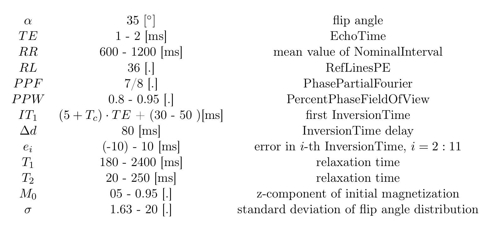
Table 2: The ranges of parameter values used to generate the training data for the NN were set with respect to the range of typical values in human tissues and the setting of the scanner used for the validation measurements. The first InversionTime was generated randomly in the given range, the others are derived from it using $$$\Delta d,RR$$$ and increment $$$e_i$$$, which is introduced to simulate the nonconstant value of $$$RR$$$ in real measurements.